
How to Apply Strikethrough to a Cell in Excel 2013
Select the cell and press Ctrl + 5, or use Ctrl + 1 > Font > Strikethrough. How to cross out part of a cell, add a button, and auto-strike done tasks.
How-to guides and tutorials to help you perform specific tasks and use the Microsoft Excel 2013 application.
Select the cell and press Ctrl + 5, or use Ctrl + 1 > Font > Strikethrough. How to cross out part of a cell, add a button, and auto-strike done tasks.

Switch Excel ruler units to centimeters in File > Options > Advanced > Display, and view the ruler in Page Layout view.

When you have information in a spreadsheet that you want to use in a document or a slideshow, then you might just copy and paste …

While many page numbering tasks will only involve one document, you might be combining your spreadsheet with something else for a project. This could mean …

Stop Excel 2013 turning addresses into links: File, Options, Proofing, AutoCorrect Options, AutoFormat As You Type, uncheck the hyperlink option.

Microsoft Excel will show you some of the files that you have been working on recently when you click the File tab at the top-left …

Looking at the formulas you type into a Microsoft Excel spreadsheet can help you troubleshoot issues that might arise if the formula isn’t working or …

Show a formula result in an Excel 2013 text box: put the formula in a cell, select the text box border, and type = plus the cell address.

Excel 2013 can hide the horizontal and vertical scroll bars for an individual workbook. This can create a cleaner worksheet view, but it also removes …

Find the formula bar in Excel, show or hide it from the View tab on Windows, Mac, and the web, expand it for long formulas, and fix a missing formula bar.

Add a hyperlink to a picture in Excel with Ctrl+K: link to a web page, another sheet, a file or an email, add a ScreenTip, and edit or remove the link.

Make text uppercase in Excel 2013 and later with the UPPER function or Flash Fill, replace the original text, and use LOWER and PROPER.

Delete a text box in Excel 2013 by selecting its border, remove several or all objects at once, and use the Selection Pane for hidden boxes.

Print a title on every page in Excel 2013 with Print Titles and Rows to repeat at top, or add it to the header, plus fixes when Print Titles is grayed out.

Hide rows and columns in Excel 2013 with right-click, the Format menu, or Ctrl + 9 and Ctrl + 0, unhide them again, and hide individual cell contents.

Remove all page breaks in Excel with Reset All Page Breaks, delete single breaks in Page Break Preview, hide dotted lines, and control breaks with scaling.

Print Excel 2013 sheets cleanly: set a print area, use landscape and narrow margins, scale to fit, repeat headers, and preview. Checklist and fixes.

Fill cells with color in Excel 2013 using the Fill Color button, Format Cells, or conditional formatting, and remove shading with No Fill.

Excel’s Live Preview shows how certain formatting choices will look when you point to them before you actually apply the change. If you find the …

Print only part of an Excel spreadsheet with Print Selection or a saved print area, print separate ranges, and fit the selection on one page.

Fill consecutive numbers in Excel 2013 by dragging the fill handle, using Home, Fill, Series, or a ROW formula for numbers that update.

Format money without a dollar sign in Excel 2013: use Comma Style, or Format Cells > Accounting with Symbol set to None. Plus removing typed $ signs.

Print without cell borders in Excel 2013: turn off printed gridlines, remove borders with No Border, clear table styles, and check lines in Print Preview.

Keep UPC codes at 12 digits in Excel with a custom format of twelve zeros. Stops lost leading zeros and scientific notation.

Remove the underline from a link in Excel 2013 with Ctrl+U or by modifying the Hyperlink cell style for all links, change link color, or remove links entirely.

Making cell selections in spreadsheet applications like Google Sheets or Microsoft Excel can be as easy as simply clicking on the cell you want. Maybe …

Change the default font in Excel 2013 under File, Options, General, then restart Excel. Also covers the Normal style for existing workbooks.

Set the print area in Excel 2013 from Page Layout > Print Area, add to it, print multiple areas, fit it on one page, and clear it.

Crop a picture in Excel with the Picture Format tab: trim edges, crop to a circle or aspect ratio, reset a crop and delete cropped areas.

Remove strikethrough in Excel with Ctrl + 5 or Format Cells, clear it from part of a cell, and fix strikethrough added by conditional formatting.

The print settings for an Excel spreadsheet are frequently an afterthought for Excel users, as the focus is on ensuring that the data in the …

Remove percentage formatting in Excel 2013 and later: switch to General, turn 35% into 35 with Paste Special Multiply, and strip % signs stored as text.

Print Excel sheets without column letters and row numbers by unchecking Headings > Print in Page Layout. Works in Excel 2013 through Microsoft 365.

Not everyone knows every formula in Microsoft Excel, and determining not only the correct formula, but the way to use it, can be difficult. Excel …

Print a blank grid in Excel 2013: set a print area over empty cells and tick Gridlines > Print, or add All Borders for darker lines.
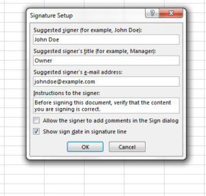
Adding a line for signatures to a Microsoft Excel document can be accomplished a couple of different ways. The first option that many will use …

Excel shows two decimals because of the cell format, not the stored value. Use Increase Decimal or Format Cells to show more digits.
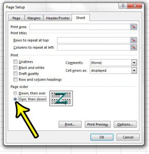
When you print a large spreadsheet in Microsoft Excel 2013, the default behavior is for the data to print down, then over. This means that …
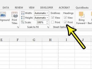
Keeping track of which data goes in which columns is often a problem for people reading printed Excel spreadsheets. The columns can start to look …

Set Page Layout as the default view in Excel 2013: File > Options > General > Default view for new sheets > Page Layout View. Plus switching views.
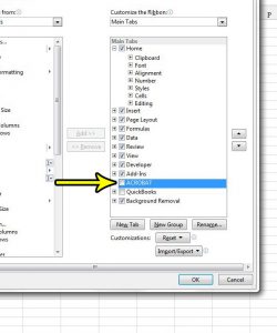
The row of buttons and tabs at the top of your Excel window is called the ribbon, and it offers an efficient way for you …
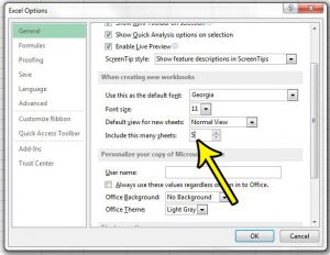
A file in Microsoft Excel is called a workbook, and that workbook can include a number of different spreadsheets called worksheets. Organizing large amounts of …
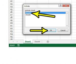
Hiding data in an Excel spreadsheet is a common practice when there is data that isn’t necessary to view, but that you either need for …
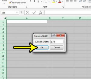
Having very wide or very skinny columns in Excel can make it difficult to work with the rest of the data in your spreadsheet. Whether …
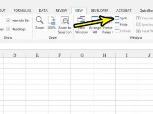
Excel 2013’s Split feature divides a worksheet window into independently scrollable panes. If you accidentally create a split or no longer need to compare distant …

Stop Excel 2013 from recalculating formulas automatically: Formulas, Calculation Options, Manual. Press F9 to recalculate when you are ready.
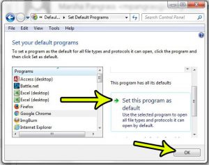
It’s not uncommon for someone to have more than one Web browser on their computer. Windows 7 includes Internet Explorer by default, but you may …

Add a gradient fill in Excel 2013: select cells, press Ctrl + 1, go to Fill > Fill Effects, pick two colors and a style. Plus shapes and charts.
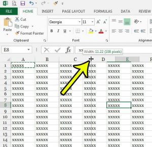
Is there a lot of information that you are trying to include in a cell in your worksheet, and you would like to make sure …

Shrink text to fit inside a cell in Excel with Format Cells > Alignment > Shrink to fit, and learn when to use Wrap text or AutoFit instead.