Often when you are working with a lot of data in Excel you will need to scroll to a point where a column or row label is no longer visible. This can usually be resolved by freezing the top row of the sheet so that you always keep the header, or title, row visible, but there is another way to visibly segment your spreadsheet. This takes advantage of the Split screen mode.
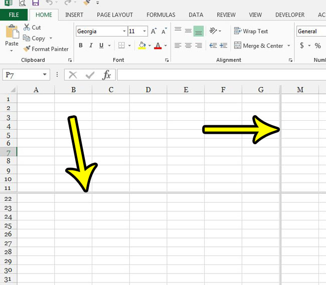
You have the Split view enabled in Excel when there are gray horizontal and vertical bars segmenting the spreadsheet. However, if you didn’t create this split screen yourself, you may find it difficult or confusing to work with. Fortunately it is something that you can remove or disable in the spreadsheet by following the guide below.
How to Stop Splitting the Screen in a Spreadsheet in Excel 2013
The steps in this article are going to assume that you currently have a spreadsheet with a split screen, and that you would like to remove it. A split screen in Excel 2013 will look similar to the image below, where there is a horizontal and a vertical bar running through the middle of the worksheet.

Note that the split screen is a setting that is specific to individual worksheets. Changing the split screen setting for a single spreadsheet will not affect other files that you work on in Excel.
Step 1: Open the file with the split screen in Excel 2013.
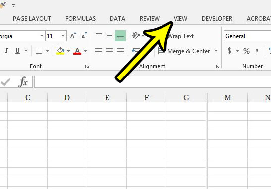
Step 2: Click the View tab at the top of the window.

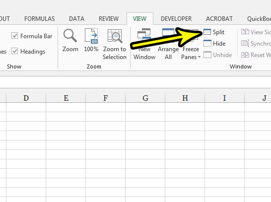
Step 3: Click the Split button in the Window section of the ribbon.

Note that you can also remove a split screen bar by double-clicking on it. This can be helpful, for example, if you wanted to keep the horizontal split screen bar, but wanted to delete the vertical one.
Are you having trouble getting your spreadsheet to print well? Read our Excel printing optimization guide for some tips and pointers that can make printing a little less of a hassle.

Kermit Matthews is a freelance writer based in Philadelphia, Pennsylvania with more than a decade of experience writing technology guides. He has a Bachelor’s and Master’s degree in Computer Science and has spent much of his professional career in IT management.
He specializes in writing content about iPhones, Android devices, Microsoft Office, and many other popular applications and devices.