While many situations might call for proper capitalization in a document, there is a benefit to knowing how to change the case of some of the content in a spreadsheet.
Microsoft Excel has a variety of proper functions that not only let you perform mathematical operations, but also change formatting.
in the case of text, you are able to have text converted to upper case letters or lower case letters with the assistance of a formula.
Our tutorial below will show you how to make all letters capital in Excel with the help of a formula that takes the text case from the original column data and then will change case for the data in a new column.
How to Make All Text Uppercase in Excel 2013
- Open the spreadsheet.
- Right-click on the column, then choose Insert.
- Type =UPPER(XX) into the first blank cell, but replace “XX” wither the cell location.
- Right-click on the uppercase cell and choose Copy.
- Paste the formula to the rest of the cells.
- Copy all of the uppercase cells.
- Right-click on the desired location, then choose Paste Values.
- Delete any remaining unwanted cells as needed.
Our guide continues below with more information on making all of your letters capital in Microsoft Excel, including pictures of these steps.
If you have ever needed to re-enter a large amount of data in a spreadsheet, then you know how tedious it can be.
This re-entry is also prone to error, and it can be frustrating to perform a lot of work simply because you need to switch some formatting.
Fortunately, you can use the =UPPER(XX) formula to convert existing text to uppercase in Excel 2013. You can then copy and paste the values from the formula to replace the existing lowercase or sentence case data.
Uppercase typing may have negative connotations when used conversationally in text messages or emails, but there are certain types of databases or situations where your data needs to be in all capital letters.
So if you have a spreadsheet of data that is all lowercase, or is a mixture of lowercase and uppercase, you may be looking for a way to make all of the text uppercase in Excel 2013.
Fortunately, you can accomplish this with the help of a formula that can automatically make all of your text uppercase.
Our guide below will show you how to use this formula, then replace your original lowercase data with the uppercase data that you need.
How to Convert to All Capital Letters in Excel 2013 (Guide with Pictures)
The steps in this guide are going to assume that you currently have a spreadsheet with some cells that are lowercase, but you would prefer to have them uppercase.
We are going to accomplish this conversion with a simple formula. The results of that formula can then be copied and pasted into the original cells, allowing you to replace the original lowercase text with the new and improved uppercase text.
Step 1: Open your spreadsheet containing the cells for which you would like to make all of the text uppercase.
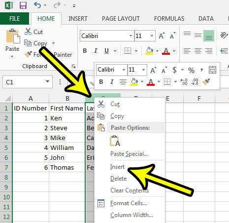
Step 2: Right-click on the column heading to the right of the column with the lowercase text, then click the Insert option.
This is going to add a new, empty column directly to the right of the column we are modifying.
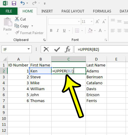
Step 2: Click inside the cell to the right of the first cell with lowercase text, then type =UPPER(XX), but replace the XX with the cell location containing the lowercase text. In this example, that is cell B2. Press Enter on your keyboard after completing the formula.
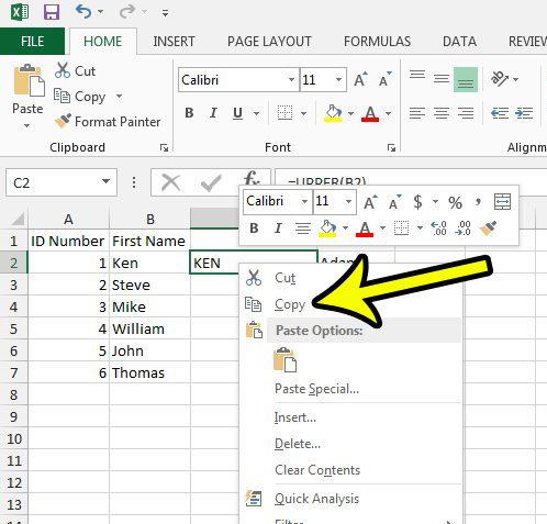
Step 3: Right-click on the cell containing the uppercase text, then click the Copy option.
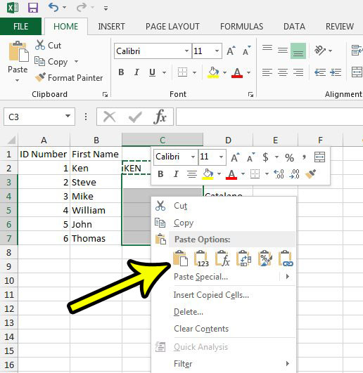
Step 4: Select the cells into which you wish to convert the original lowercase text to uppercase text, then right-click one of the selected cells and select the Paste option.
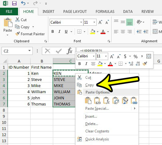
Step 5: Select all of the cells that now contain uppercase text, then right-click on one of them and select the Copy option.
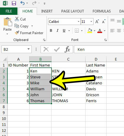
Step 6: Select the original cells that still contain the lowercase text.
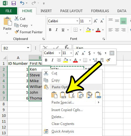
Step 7: Right-click on the selected cells, then click the Paste option with the numbers on it.
This is going to allow you to paste the values from the formulas rather than the formulas themselves.
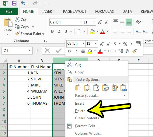
Step 8: Delete the column that contains the formulas by right-clicking the column heading, then clicking the Delete option.
Now that you know how to capitalize all letters in Excel you will be able to make that conversion whenever you have data in your cell that you need to be uppercase instead of lowercase.
You can continue below for additional discussion on changing the case of your cell data in Microsoft Excel.
More Information on How to Make Text All Caps in Excel 2013
Note that the data that is being displayed via this formula is still formula data before you go through the process of copying and pasting it as values.
This means that it interacts with cell adjustments the same way as a SUM or other formula type would. For example, if you were to add or delete rows while the cells still contained formulas, then the displayed results would adjust accordingly.
If you copy and paste the uppercase text from Excel to another program, like Microsoft Word, then it will be pasted as values automatically. In some cases, it can be easier to use the Excel capitalize all formula rather than trying to perform the same task in a Word document.
You can use similar Excel functions that we used in this guide on how to make font all caps in Excel if you want to convert text to something other than upper case, such as proper case.
In that situation, you would use the =PROPER formula instead. This proper function can come in handy when you are working with a lot of lowercase letters, for example.
If you aren’t only interested in using a cell reference for how to capitalize in Excel for a small amount of Excel data, but would instead like to make the change for an entire column, then you can enter the formula into the formula bar for the first cell in the column, then click on the handle at the bottom-right corner of that cell and drag it down to fill the rest of the column.
Working With Large Amounts of Excel Data
It is not uncommon to find oneself working with many Excel files when dealing with huge volumes of data. Combining data from various files into a single file can be a time-consuming operation, but it is also necessary for data analysis and decision-making. In this tutorial, we’ll go through the fundamentals of integrating data from various Excel files into a single file.
Do you have a lot of CSV files that you need to combine into one file, but you are looking for a better way to do it than cutting and pasting? Learn how to merge CSV files with the Windows command prompt and make it much easier to combine your data into one spreadsheet.
Data Combination Using Copy and Paste
The copy and paste method is one method for combining data from various Excel files. To begin, open the first Excel file and choose the range of cells you want to copy. Right-click on the selected cells and pick “Copy” from the context menu. Then, open the second Excel file and choose the cell where you want to paste the copied data. Right-click the cell and select “Paste” from the context menu. Repeat this method for each Excel file until all of the data is integrated into a single file.
Consolidating Data Using the Consolidate Function
Another option to merge data from numerous Excel files is to use the consolidate function. This function allows you to combine data from many ranges and sheets into a single range or sheet. Follow these steps to use the consolidate function:
- Open the Excel file where you wish to merge the data.
- “Data” > “Consolidate”
- Select the function to use to consolidate the data in the Consolidate dialog box, such as sum, average, or count.
- Select the range of cells from each Excel file in the “Reference” section.
- Click “Add” to add the selected range to the “All references” section.
- Repeat steps 4-5 for each Excel file you want to consolidate.
- To consolidate the data, click the “OK” button.
Combining Data using Power Query
Power Query is a sophisticated tool that can be used to aggregate data from several Excel files. To utilize Power Query, go through the following steps
- Open Excel and go to “Data” > “Get Data” > “From File” > “From Folder.”
- Select the folder containing the Excel files that you want to combine in the “From Folder” dialog box.
- Click “Edit” to open the Power Query Editor.
- Select the first Excel file to merge in the Power Query Editor.
- Click “Transform Data” > “Keep Rows” > “Keep All Rows.”
- Repeat steps 4-5 for each Excel file you want to integrate.
- Click “Close & Load” to merge the data.
Finally, merging data from various Excel files is a critical activity for data analysis and decision-making. Whether you utilize copy and paste, the consolidate function, or Power Query, it’s important to understand each method and when to apply it. By taking the time to integrate your data into a single file, you may successfully manage and manipulate your data in a way that matches your individual needs. The ability to merge data from various Excel files is a vital talent to have, whether you are working on a personal project or as part of your employment.
Frequently Asked Questions About How to Make All Letters Capital in Excel
Is there a way to change data in Excel so that the first letter in my calculated column is capital?
Yes, the change case button in Microsoft Word is good for this, but, unfortunately, it’s not available in Microsoft Excel.
Therefore you will need to use the Proper case formula.
Create a new column next to the original data, then type the formula =PROPER(XX), but replace the XX with the cell location.
You can then click and drag the bottom-right handle down to flash fill additional cells with the same formula.
How do I change text in Excel so that it has a line through it?
Microsoft Excel has a strkethrough option, though it’s not very easy to find.
Select the cells to which you wish to add a line through, then select the Home tab at the top of the window.
Click the small square button at the bottom-right of the Font group, then check the Strikethrough box.
Note that there are also Superscript and Subscript options here as well, which you can use in a similar manner.

Kermit Matthews is a freelance writer based in Philadelphia, Pennsylvania with more than a decade of experience writing technology guides. He has a Bachelor’s and Master’s degree in Computer Science and has spent much of his professional career in IT management.
He specializes in writing content about iPhones, Android devices, Microsoft Office, and many other popular applications and devices.