To apply strikethrough to a cell in Excel 2013, select the cell and press Ctrl + 5. Press it again to remove the line. You can also press Ctrl + 1 to open Format Cells, click the Font tab, check Strikethrough under Effects, and click OK. Excel 2013 doesn’t have a strikethrough button on the ribbon, but you can add one to the Quick Access Toolbar.
These steps also work in Excel 2016, 2019, 2021, 2024, and Microsoft 365. Below you’ll find how to cross out part of a cell, add a strikethrough button, and cross out tasks automatically.
Method 1: Use the keyboard shortcut
- Select the cell or range of cells.
- Press Ctrl + 5.
Use the 5 key in the row above the letters, not the number pad. On a Mac, press Command + Shift + X.
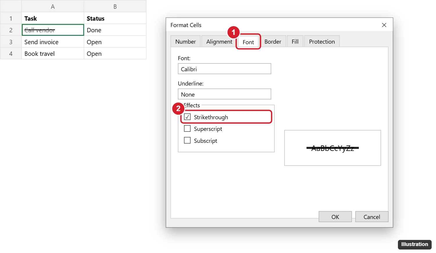
Method 2: Use Format Cells
- Select the cells.
- Press Ctrl + 1, or right-click and choose Format Cells.
- Click the Font tab.
- Under Effects, check Strikethrough.
- Click OK.
How to strike through part of a cell
- Double-click the cell, or select it and press F2.
- Select the words you want to cross out.
- Press Ctrl + 5, or press Ctrl + 1 and check Strikethrough.
- Press Enter.
This only works on text. For cells with numbers or formulas, strikethrough applies to the whole cell.
Add a strikethrough button to the Quick Access Toolbar
- Click the small down arrow at the end of the Quick Access Toolbar, at the top left of the window.
- Click More Commands.
- Under Choose commands from, select Commands Not in the Ribbon.
- Click Strikethrough, then Add, then OK.
Now you can click the button to cross out selected cells.
Cross out a task automatically with conditional formatting
If you have a to-do list with a status column, Excel can cross out finished tasks for you.
- Select the task rows, for example A2:B20.
- Click Home > Conditional Formatting > New Rule.
- Choose Use a formula to determine which cells to format.
- Type
=$B2="Done", using your status column. - Click Format, check Strikethrough on the Font tab, and click OK twice.
In newer versions of Excel, you can pair this with checkboxes: =$C2=TRUE.
Strikethrough in other versions of Excel
| Version | How |
|---|---|
| Excel 2010 to 2024 and Microsoft 365 (Windows) | Ctrl + 5 or Ctrl + 1 > Font > Strikethrough |
| Excel for Mac | Command + Shift + X, or the abc button on the Home tab |
| Excel for the web | Ctrl + 5, or the strikethrough button in the Font group |
| Excel for iPhone, iPad, and Android | Tap the cell, open Home, and tap the strikethrough button |
Frequently asked questions
Why doesn’t Ctrl + 5 work?
You may be pressing 5 on the number pad, or another app may use that shortcut. Use the 5 key above the letters, or use Format Cells.
How do I remove strikethrough?
Select the cells and press Ctrl + 5 again, or uncheck Strikethrough in Format Cells. Home > Clear > Clear Formats removes it along with other formatting.
Does strikethrough change the cell’s value?
No. It only changes how the cell looks. Formulas still use the value.
Can I use a double strikethrough in Excel?
No. Excel only has single strikethrough. Word has a double strikethrough option.

Kermit Matthews is a freelance writer based in Philadelphia, Pennsylvania with more than a decade of experience writing technology guides. He has a Bachelor’s and Master’s degree in Computer Science and has spent much of his professional career in IT management.
He specializes in writing content about iPhones, Android devices, Microsoft Office, and many other popular applications and devices.