How to Use Conditional Formatting in Excel

To use conditional formatting in Excel, select the cells you want to watch, go to Home > Conditional Formatting, pick a rule such as Highlight Cells Rules > Greater Than, enter the value to compare against, choose a format, and click OK. Excel then colors every cell that meets the condition and updates the colors automatically whenever the numbers change. For anything the preset rules can’t do, such as coloring an entire row, choose New Rule > Use a formula to determine which cells to format.

Rules that fill cells can also hide the grid, and fixing missing gridlines in Excel covers how to spot that.

This guide walks through every type of rule (highlight rules, top and bottom rules, data bars, color scales, and icon sets), shows how to write formula rules that highlight whole rows, and explains the Rules Manager, where most of the confusion happens. You’ll also find steps for Excel for Mac and Excel for the web, a worked example you can rebuild, and fixes for rules that don’t seem to work.

What you need and which versions this covers

• Excel for Microsoft 365 on Windows is the main version described here. Microsoft’s instructions apply equally to Excel 2024, 2021, 2019, and 2016 for Windows, which use the same Home tab menu and dialog boxes.
• Excel for Mac (Microsoft 365, 2024, and 2021) has the same rule types, but a few dialog boxes look different. See the Mac section.
• Excel for the web uses a Conditional Formatting task pane instead of dialog boxes. See the web section.
• A workbook you can edit. If the file opens in Protected View or as read-only, click Enable Editing first, or the Conditional Formatting button may be unavailable.
• Data in a normal range or an Excel table. Rules work on numbers, text, and dates, but some rule types only make sense for numbers.

Conditional formatting only changes how cells look. It never changes the values or formulas inside them, so you can experiment safely and remove rules at any time.

How conditional formatting works

A conditional formatting rule has three parts: the cells it watches, a condition, and a format. The cells are listed in the rule’s Applies to box. The condition is a test such as “greater than 500” or “contains the word Late.” The format is whatever Excel should apply when the test is true: a fill color, font color, bold text, a border, or a number format. Visual rule types such as data bars work slightly differently, because they draw a bar, color, or icon in every cell based on where its value falls in the range.

Because the condition is checked again every time the worksheet recalculates, the formatting is “live.” If a sales figure drops below target, its cell turns red on its own. That is the big difference from manually filling a cell with color, which stays put no matter what the cell contains. If you only need to color a few cells once, regular formatting is simpler; our guide on how to format Excel cells covers fills, fonts, and number formats.

A few terms you’ll see in the menus:

• Highlight Cells Rules: quick comparisons such as Greater Than, Between, Text that Contains, A Date Occurring, and Duplicate Values.
• Top/Bottom Rules: rank-based rules such as Top 10 Items, Bottom 10%, and Above Average.
• Data Bars, Color Scales, Icon Sets: visual rules that show every value’s size relative to the others.
• Rules Manager: the Conditional Formatting Rules Manager dialog box, where you see, edit, reorder, and delete rules.
• Precedence: the order rules are checked in. When two rules try to set the same property, such as fill color, the rule higher in the list wins.

Sample data used in this guide

The examples below use a small order tracker in cells A1:F9. You can type it into a blank sheet to follow along. Column E holds due dates, so the date-based results you see will depend on today’s date.

Row	A: Order	B: Customer	C: Region	D: Amount	E: Due date	F: Status
2	1001	Alex Rivera	West	1,250	10/02/2026	Shipped
3	1002	Jordan Lee	East	480	10/09/2026	Late
4	1003	Priya Shah	North	2,900	10/20/2026	Open
5	1004	Sam Carter	East	760	10/05/2026	Late
6	1005	Maria Gomez	South	1,980	10/28/2026	Open
7	1006	Chris Nolan	West	320	10/01/2026	Shipped
8	1007	Taylor Brooks	North	1,540	10/15/2026	Open
9	1008	Jamie Park	South	2,150	10/11/2026	Late

Method 1: Highlight cells with a preset rule (Windows)

Preset rules are the fastest way to start. This example highlights every order amount over 1,500.

Step 1: Select the cells to format

Drag across D2:D9. Select only the data, not the header in row 1, so the header isn’t included in comparisons. To format a whole column that will keep growing, you can click the column letter instead, but a defined range (or an Excel table) keeps the sheet faster and easier to manage.

Step 2: Open the Conditional Formatting menu

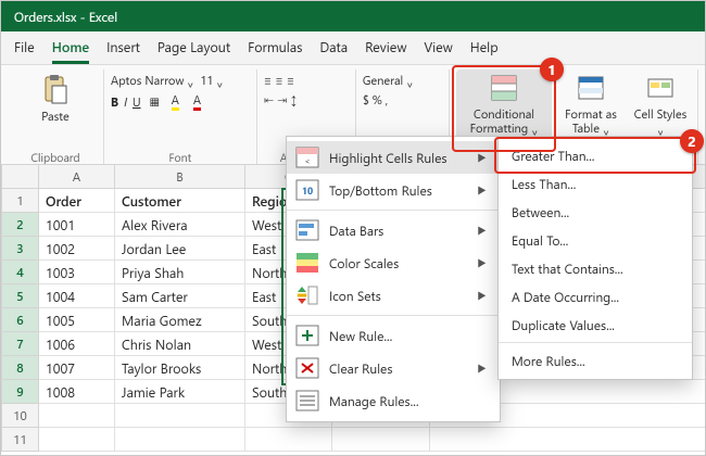
On the Home tab, in the Styles group, click Conditional Formatting. A menu opens with Highlight Cells Rules, Top/Bottom Rules, Data Bars, Color Scales, and Icon Sets at the top, and New Rule, Clear Rules, and Manage Rules at the bottom. If your Excel window is narrow, the Styles group may be collapsed into a single button; click it to reveal Conditional Formatting.

Step 3: Choose a comparison

Point to Highlight Cells Rules and click Greater Than. The other choices in this submenu are Less Than, Between, Equal To, Text that Contains, A Date Occurring, and Duplicate Values. Each opens a small dialog box with the same layout: a value box on the left and a format list on the right.

Step 4: Enter the value and pick a format

Type 1500 in the left box. You can also click a cell instead of typing, which links the rule to that cell; if you later change the number in that cell, the highlighting updates. In the with list on the right, choose a preset such as Light Red Fill with Dark Red Text or Green Fill with Dark Green Text. Excel previews the result on the sheet while the dialog box is open. Choose Custom Format at the bottom of the list to pick your own fill, font, or border.

Step 5: Click OK and test it

Click OK. In the sample data, 2,900, 1,980, 1,540, and 2,150 are highlighted. Change 480 in D3 to 1600 and press Enter: the cell is highlighted immediately. That instant update is how you know the rule is working.

Other preset comparisons worth knowing

• Between: two boxes for a low and high value. Both ends are included, so “between 500 and 1000” highlights 500 and 1000 too.
• Text that Contains: matches part of a cell’s text. Typing Late on F2:F9 highlights the three late orders. The match is not case-sensitive.
• A Date Occurring: choices such as Yesterday, Today, Tomorrow, In the last 7 days, Last week, This week, Next week, Last month, This month, and Next month. These rules compare against your computer’s current date, so results change from day to day.
• Duplicate Values: highlights values that appear more than once in the selection. Switch the first list to Unique to highlight values that appear only once instead. Microsoft notes that this rule treats * and ? as wildcard characters.

Every submenu ends with More Rules, which opens the full New Formatting Rule dialog box with the same rule already chosen, so you can fine-tune it.

Top/Bottom rules and above or below average

Top/Bottom rules compare each cell to the rest of the selection instead of to a fixed number. That makes them useful when you want “the five biggest orders” no matter what the amounts are.

1. Select D2:D9.
2. Click Home > Conditional Formatting > Top/Bottom Rules.
3. Choose one of Top 10 Items, Top 10%, Bottom 10 Items, Bottom 10%, Above Average, or Below Average.
4. For the item and percent rules, change the number in the spin box. “Top 10 Items” is just the default name; set it to 3 to highlight the three largest values.
5. Pick a format and click OK.

In the sample data, Top 3 Items highlights 2,900, 2,150, and 1,980. Above Average compares each amount to the average of D2:D9 (1,422.50 here) and highlights the four orders above it. If you need “one or two standard deviations above the average,” choose More Rules and select the option you want in the list under Format values that are.

Ties are included. If the third and fourth largest values are equal, a Top 3 rule highlights both, so you may see more highlighted cells than the number you entered.

Data bars, color scales, and icon sets

These three rule types don’t pick out a subset of cells. They format every cell in the range so you can compare values at a glance, a bit like a chart inside the cells.

Data bars

Select D2:D9 and click Home > Conditional Formatting > Data Bars, then choose a Gradient Fill or Solid Fill color. Each cell gets a horizontal bar whose length reflects its value: the largest amount gets the longest bar. Solid fill is usually easier to read when the cells also show numbers.

To adjust the bars, open Manage Rules, select the data bar rule, and click Edit Rule. There you can set what counts as the shortest and longest bar (Automatic, Lowest Value, Number, Percent, Percentile, or Formula), check Show Bar Only to hide the numbers, add a border, change the bar direction, and use Negative Value and Axis to control how negative numbers are drawn.

Color scales

Click Home > Conditional Formatting > Color Scales and choose a scale. A two-color scale shades from one color to another; a three-color scale adds a middle color. Hover over each option to see which is which. With the Green – Yellow – Red scale, high values are green, middle values yellow, and low values red. If lower numbers are better in your data (costs, delays, error counts), pick a scale with the colors reversed so green still means good.

In Edit Rule you can switch between 2-Color Scale and 3-Color Scale and set the minimum, midpoint, and maximum by Lowest/Highest Value, Number, Percent, Percentile, or Formula. Percentile is a good choice when one extreme value would otherwise wash out the colors for everything else.

Icon sets

Click Home > Conditional Formatting > Icon Sets and choose a set such as 3 Arrows, 3 Traffic Lights, or 5 Ratings. Excel sorts the values into three to five groups and shows an icon for each group. By default, a three-icon set splits the range by percent of the range: values at 67% and above get the first icon, values from 33% get the middle icon, and the rest get the last icon.

Those default thresholds are based on the spread of your numbers, not on targets you care about. To use real cutoffs, open Edit Rule, change Type from Percent to Number, and type the values, for example 2000 for the green icon and 1000 for yellow. Edit Rule also has Reverse Icon Order and Show Icon Only. Icons scale with the cell’s font size, so you may need to widen the column.

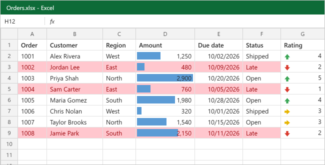
The illustration below adds a Rating column (G) with scores from 1 to 5 and applies the default 3 Arrows set. Because the scores span 1 to 5, the 67% cutoff falls at about 3.7 and the 33% cutoff at about 2.3: scores of 4 and 5 get green up arrows, 3 gets a yellow sideways arrow, and 1 and 2 get red down arrows.

You can sort or filter by these formats. Right-click a formatted cell, point to Sort or Filter, and choose the cell color, font color, or icon you want at the top.

The Quick Analysis shortcut

When you select a range of data, a small Quick Analysis button appears at its lower-right corner. Click it or press Ctrl+Q, then open the Formatting tab and hover over each choice to preview it. For numbers, the choices are Data Bars, Colors (color scales), Icon Sets, Greater, Top 10%, and Clear. For text, they are Text, Duplicate, Unique, Equal To, and Clear. Quick Analysis offers fewer options than the ribbon, but it’s handy for a fast look. The button doesn’t appear when the selected cells are empty, or when only the top-left cell has data.

Method 2: Formula rules and highlighting a whole row

Preset rules can only format the cell that meets the condition. If you want the entire row for a late order to turn red, or a cell to change color based on a different column, you need a formula rule. The formula must return TRUE or FALSE. Excel applies the format wherever the result is TRUE.

Step 1: Select every cell that should change color

To shade whole rows, select A2:F9, starting from A2 so that A2 is the active cell (the white cell in the selection). The active cell matters because you’ll write the formula as if it were for that one cell.

Step 2: Open New Rule

Click Home > Conditional Formatting > New Rule. The New Formatting Rule dialog box opens with a Select a Rule Type list at the top.

Step 3: Choose the formula rule type

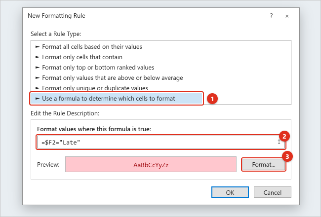
Click Use a formula to determine which cells to format, the last item in the list. The lower half of the dialog box changes to show a box labeled Format values where this formula is true.

Step 4: Type the formula for the first row

Type =$F2="Late". The dollar sign before F locks the column, so every cell in the row looks at the Status column. Leaving the row number unlocked lets Excel move the test down one row at a time: row 3 checks F3, row 4 checks F4, and so on. Always start the formula with an equal sign, and put text in straight double quotes.

If you click a cell while the formula box is active, Excel inserts a fully locked reference such as $F$2. That locks the row too, so every row would check F2 only. Press F4 to cycle through reference types until you see $F2, or edit the text by hand.

Step 5: Pick the format

Click Format. In the Format Cells dialog box, use the Fill tab for a background color and the Font tab for color, bold, or strikethrough, then click OK. The Preview box in the New Formatting Rule dialog box shows your choice instead of “No Format Set.”

Step 6: Apply and check

Click OK. Rows 3, 5, and 9 are shaded across all six columns. Change Status in F4 to Late and row 4 joins them. If nothing is highlighted, the most common cause is the dollar sign in the wrong place or a formula written for a row other than the active cell’s row; see Troubleshooting.

Useful formula rules

Each formula below assumes the selection starts in row 2. Adjust the row number to match the first row you select.

Goal	Select	Formula
Shade rows where the amount is over 2,000	A2:F9	=$D2>2000
Flag overdue orders that aren’t shipped	A2:F9	=AND($E2<TODAY(),$F2<>"Shipped")
Orders due within the next 7 days	E2:E9	=AND(E2>=TODAY(),E2<=TODAY()+7)
East or West region	C2:C9	=OR(C2="East",C2="West")
Compare with a target typed in H1	D2:D9	=D2>=$H$1
Duplicate customers (formula version)	B2:B9	=COUNTIF($B$2:$B$9,B2)>1
Blank cells that should have data	A2:F9	=ISBLANK(A2)
Shade every other row	A2:F9	=ISEVEN(ROW())

You don’t need to wrap these tests in IF. =$D2>2000 already returns TRUE or FALSE, so =IF($D2>2000,TRUE,FALSE) only adds clutter. Formulas can also refer to cells on another worksheet in the same workbook. If you want to learn more about COUNTIF before using it here, see how to count a word in Excel.

Formula rules aren’t limited to color. A common use is a to-do list where finished items are crossed out automatically: set the format’s font to strikethrough. Our guide to strikethrough in Excel covers that setup.

The other rule types in New Rule

The Select a Rule Type list has six entries. Besides the formula option, they are Format all cells based on their values (color scales, data bars, icon sets), Format only cells that contain (cell value, specific text, dates, blanks, no blanks, errors, no errors), Format only top or bottom ranked values, Format only values that are above or below average, and Format only unique or duplicate values. “Format only cells that contain” is the quickest way to highlight blanks or error values such as #N/A without writing a formula.

Manage, edit, and reorder rules

Every rule you create is stored in the Conditional Formatting Rules Manager. Open it with Home > Conditional Formatting > Manage Rules.

See all of the rules

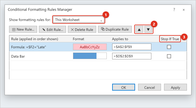
The Show formatting rules for list at the top starts on Current Selection, which only lists rules that touch the cells you had selected. If the list looks empty or incomplete, switch it to This Worksheet. You can also pick another sheet or a table from the same list.

Edit, duplicate, or delete a rule

Select a rule and click Edit Rule to change its condition or format. Duplicate Rule makes a copy you can modify, which is quicker than starting over for a similar rule. Delete Rule removes the selected rule. The change isn’t final until you click OK or Apply, so Cancel backs out of a mistake.

Change the cells a rule applies to

Click in the Applies to box for a rule and type a new range, such as =$A$2:$F$200, or select it on the sheet. This is the cleanest way to extend a rule to new rows. If you change the range of a formula rule, keep the formula written for the first cell of the new range.

Rule order and conflicts

Rules are checked from top to bottom, as the column heading Rule (applied in order shown) suggests. New rules are added at the top. When two true rules set different things, such as one making text bold and the other filling the cell yellow, the cell gets both. When they set the same thing, such as two different fill colors, only the higher rule’s format appears. Select a rule and use the Move Up and Move Down arrow buttons to change the order.

For example, if you have a red fill for “overdue” and a yellow fill for “due within 7 days,” put the overdue rule first. Otherwise, a date that matches both conditions shows yellow.

What Stop If True does

Checking Stop If True on a rule tells Excel not to check any rules below it for cells where that rule is true, even rules that wouldn’t conflict. Use it when you want one rule to have the final say. A typical case: you have an icon set on a column but don’t want icons on rows that are already marked Shipped. Create a formula rule such as =$F2="Shipped" with no format set, place it above the icon set, and check Stop If True. Microsoft also describes Stop If True as a way to simulate how older Excel versions that supported only three rules would display the sheet.

Conditional formatting versus manual formatting

If a cell has both a manual fill and a conditional fill, the conditional fill is what you see while the rule is true. The manual format is still there underneath and reappears when the rule is false or deleted. Manual formatting doesn’t appear in the Rules Manager.

Copy, find, and clear conditional formatting

Copy rules to other cells

• Format Painter: click a formatted cell, click Home > Format Painter, and drag across the destination cells. Double-click Format Painter to paint several areas, then press Esc to stop.
• Paste formatting only: copy the formatted cells with Ctrl+C, select the destination, then choose Home > Paste > Formatting (or Paste Special > Formats).

Copying, pasting, and filling cells that have conditional formatting creates new rules based on the source cells. Over time, this can leave many near-identical rules with broken-up Applies to ranges, which makes the sheet slower and confusing. When that happens, open the Rules Manager on This Worksheet, keep one rule, set its Applies to box to the full range, and delete the duplicates. If a copied formula rule uses relative references, check that they still point where you expect.

Find cells that have conditional formatting

To select every cell on the sheet with a rule, click Home > Find & Select > Conditional Formatting. To find only the cells that share one rule, click a cell with that rule, choose Home > Find & Select > Go To Special, select Conditional formats, then Same, and click OK.

Clear rules

Choose Home > Conditional Formatting > Clear Rules, then Clear Rules from Selected Cells or Clear Rules from Entire Sheet. You can also clear rules from a table or PivotTable when one is selected. To remove a single rule and keep the others, delete it in the Rules Manager instead. If you clear rules by mistake, press Ctrl+Z right away to undo.

Note that Home > Clear > Clear Formats removes conditional formatting along with every other format in the selection, including number formats and borders. If you only want the rules gone, use Clear Rules.

Excel for Mac

Excel for Mac has the same rule families on the Home tab. Microsoft’s Mac instructions describe these paths:

Step 1: Apply a preset rule

Select the cells, click Home > Conditional Formatting, and point to Highlight Cells Rules, Top/Bottom Rules, Data Bars, Color Scales, or Icon Sets. Choose a rule, set the value and format, and click OK.

Step 2: Create a formula rule

Click Home > Conditional Formatting > New Rule. In the Style list, choose Classic. In the list below it, change the rule type to Use a formula to determine which cells to format. Type the formula (for example =$F2="Late") in the next box, then open the Format with list and choose the custom format option to pick colors in Format Cells. Click OK. The reference rules are the same as on Windows: write the formula for the first selected cell and lock columns with $ as needed.

Step 3: Manage, find, and clear rules

Choose Home > Conditional Formatting > Manage Rules to edit or delete rules. Select a rule and click Edit Rule, or select it and use the delete button (its tooltip reads “Click to delete selected rule”) to remove it. To find formatted cells, use Edit > Find > Go To, click Special, and choose Conditional formats. To remove rules, use Home > Conditional Formatting > Clear Rules.

Microsoft’s support article for Excel for Mac covers highlighting patterns and trends with conditional formatting if your dialog boxes look different from these steps.

Excel for the web

Excel for the web uses a Conditional Formatting task pane on the right side of the window instead of pop-up dialog boxes.

Step 1: Apply a preset rule

Select the cells, then choose Home > Conditional Formatting and pick from Highlight Cell Rules, Top/Bottom Rules, Data Bars, Color Scales, or Icon Sets.

Step 2: Create a formula rule

Choose Home > Conditional Formatting > New Rule. In the pane, check the Apply to range box, set Rule Type to Formula, type the formula, choose a format, and click Done.

Step 3: Manage and clear rules

Choose Home > Conditional Formatting > Manage Rules. The pane lists rules for the current selection; change the scope list to this sheet to see everything. Hover over a rule and select the pencil icon to edit it, use the plus sign to add a rule, or use the trash can to delete one or all rules. Clear Rules on the menu works the same way as on Windows.

Rules created in the web version are saved with the workbook, so they also work when you open the file in the desktop app. If an option you need, such as a specific data bar setting, isn’t in the pane, open the file in the desktop app with Editing > Open in Desktop App and finish the rule there.

Worked example: an order tracker

Here’s how the pieces fit together on the sample data. The goal: late orders stand out, big orders are easy to spot, and amounts are easy to compare.

1. Whole-row highlight for late orders. Select A2:F9, choose New Rule > Use a formula to determine which cells to format, enter =$F2="Late", and choose a light red fill. Rows 3, 5, and 9 turn red.
2. Data bars on Amount. Select D2:D9 and choose Data Bars > Solid Fill > blue. The 2,900 order has the longest bar and the 320 order the shortest.
3. Bold for big orders. With D2:D9 still selected, choose Highlight Cells Rules > Greater Than, enter 2000, choose Custom Format, and set the font to bold. Orders 1003 and 1008 are bold. Because bold doesn’t conflict with the red fill or the bars, all three rules show together in row 9.
4. Check the order. Open Manage Rules, switch to This Worksheet, and confirm all three rules are listed with the correct Applies to ranges.
5. Extend it. When you add orders in rows 10 to 50, edit each rule’s Applies to box to end at row 50, or convert the data to a table with Insert > Table before adding rules so new rows are easier to include.

The result is a sheet where you can find late orders, the largest orders, and the overall spread of amounts without reading every number. You can then sort by cell color to bring late orders to the top.

Troubleshooting

The rule highlights the wrong cells or nothing at all

For formula rules, this is almost always a reference problem. Excel reads the formula as written for the active cell of the selection. If you selected A2:F9 but wrote =$F1="Late", every row checks the row above it. Rewrite the formula for the first row of the range. Also check the dollar signs: $F$2 makes every cell check F2, while F2 without a dollar sign shifts columns too, so a whole-row rule would check F, G, H, and so on.

Numbers aren’t highlighted even though they look larger

The cells may contain numbers stored as text, often from imported data. A green triangle in the cell corner is a common sign. Select the cells, click the warning icon, and choose Convert to Number, then the rule will treat them as numbers.

Cells with errors aren’t formatted

If a cell’s formula returns an error such as #DIV/0!, Microsoft notes that the conditional format isn’t applied to it. Wrap the cell formula in IFERROR, for example =IFERROR(B2/C2,0), or add a separate rule using “Format only cells that contain” with Errors to highlight them.

Only one of two rules shows

Two rules are setting the same property, such as fill color, and the higher one wins. Open the Rules Manager and reorder them, or check whether Stop If True is turned on for the upper rule.

The Rules Manager seems empty

The Show formatting rules for list is probably set to Current Selection, and the selected cells have no rules. Switch it to This Worksheet.

The Conditional Formatting button is grayed out

Check whether the file is open in Protected View or read-only (click Enable Editing), whether the sheet is protected (Review > Unprotect Sheet, if you know the password), and whether you’re in the middle of editing a cell (press Esc). Selecting several sheet tabs at once can also limit what’s available, so click a single tab.

The workbook got slow after lots of copying

Repeated copy and paste can create dozens of duplicate rules. Consolidate them in the Rules Manager as described in Copy, find, and clear, and avoid applying rules to entire columns when your data uses only a few hundred rows.

Date rules changed overnight

Rules using A Date Occurring or TODAY() are designed to change as the date changes. That’s expected. If you need fixed dates, type the date into a cell and compare against that cell instead.

Frequently Asked Questions

Can conditional formatting highlight a cell based on another cell?

Yes. Select the cells to color, choose New Rule > Use a formula to determine which cells to format, and refer to the other cell in the formula. For example, select B2:B9 and use =$D2>1500 to color customer names when their order amount is over 1,500.

How many rules can one range have?

Current Excel versions allow many rules on the same range, well beyond the three-rule limit of very old versions. In practice, keep the number small so the rules stay easy to understand and the sheet stays fast.

Does conditional formatting change my data?

No. Rules only change how cells look. Values, formulas, sorting, and calculations are unaffected, and clearing the rules returns the cells to their regular formatting.

How do I color a cell when it’s blank?

Select the range, choose New Rule, pick Format only cells that contain, change Cell Value to Blanks, click Format, and choose a fill. Cells that contain a formula returning empty text (“”) may not count as blank; for those, use the formula rule =A2="" instead.

Can I use conditional formatting in a PivotTable?

Yes, in Excel for Windows. Rules on a PivotTable stay in place when you filter or rearrange it, as long as the underlying fields remain. Some rules, such as unique or duplicate values, can’t be used on fields in the Values area.

Why does the Duplicate Values rule miss some duplicates?

Values must match exactly apart from letter case. Extra spaces, numbers stored as text versus real numbers, or slightly different spellings make cells look the same without being identical. Clean the data with TRIM or Convert to Number, or use a COUNTIF formula rule.

Is conditional formatting the same in Google Sheets?

The idea is the same, but the menus differ: Google Sheets uses Format > Conditional formatting and a side panel. See how to highlight in Google Sheets for those steps.

Will my rules work if I share the file?

Yes. Rules are saved in the .xlsx file and work in Excel for Windows, Mac, and the web. If you save in an older format such as .xls, newer rule options may be lost or simplified, so keep .xlsx when possible.

Next steps

Start with one preset rule on a column you check often, then try a whole-row formula rule using the =$F2="Late" pattern with your own column and value. Once you have more than two rules, open the Rules Manager on This Worksheet to confirm their order. For every option and setting, Microsoft’s guide on using conditional formatting to highlight information in Excel is the official reference, and its companion page on data bars, color scales, and icon sets goes deeper into those visual rules.