How to Create a Drop-Down List in Excel

To create a drop-down list in Excel, type the choices you want in a column of cells, select the cell or cells that should get the list, and go to Data > Data Validation. On the Settings tab, set Allow to List, click in the Source box and select your list of choices, then click OK. A small arrow now appears whenever someone selects one of those cells, and they can pick an entry instead of typing it. For a quick list of two or three fixed options, you can skip the cells and type the choices straight into the Source box, separated by commas, such as Yes,No,Maybe.

That’s the whole basic method. The rest of this guide shows how to build it step by step, how to make the list grow automatically when you add items, how to keep the choices on a hidden sheet, how to build a second list that changes based on the first, and what to do when the arrow doesn’t show up or Excel won’t accept the source. A drop-down works best from a clean source list, so remove duplicate entries from that list first.

What you need and which versions this covers

• Excel for Microsoft 365 on Windows is the version used for the main steps and illustrations. Excel 2024, 2021, 2019, and 2016 for Windows use the same Data > Data Validation command and the same dialog box.
• Excel for Mac (Microsoft 365, 2024, and 2021) works the same way, but the command may be labeled Data Validation or Validate. See the Mac section.
• Excel for the web can create drop-down lists too, with slightly different checkbox names. See the Excel for the web section.
• Formula-based lists that use UNIQUE, SORT, FILTER, or the # spill reference need Excel for Microsoft 365, Excel 2024, Excel 2021, or Excel for the web. Excel 2019 and 2016 need the older formulas shown later.
• A worksheet you can edit. If the sheet is protected or the workbook is shared in the old “Shared Workbook” mode, the Data Validation button is unavailable until you unprotect or stop sharing it.

Two terms come up a lot. Data validation is the Excel feature that controls what can be entered in a cell; a drop-down list is just one kind of validation rule (the “List” kind). The source is where the list’s choices come from: either text you type in the dialog box or a reference to cells that hold the choices. Pair the drop-down with an XLOOKUP formula so picking an item fills in its price or details automatically.

Choose where your list items will live

Every Excel drop-down list is built in the same dialog box. The only real decision is where the choices are stored, because that decides how easy the list is to change later. Use this table to pick an approach before you start.

Source type	What goes in the Source box	Grows when you add items?	Best for
Typed items	Yes,No,Maybe	No. You edit the dialog box each time.	Two to five choices that rarely change
Range of cells	=$E$2:$E$6	Only if you insert new cells inside the range	A fixed list you want to see on the sheet
Excel table column	The table’s data cells, selected with the mouse	Yes, automatically	Most lists, especially ones that grow
Named range	=Categories	Only if the name points to a table or formula	Lists reused in many places or workbooks shared with others
Formula or spill range	=$H$2# or an OFFSET formula	Yes	Sorted, duplicate-free, or dependent lists

If you’re not sure, put the items in a column, turn that column into an Excel table, and point the drop-down at the table. Microsoft recommends this too, because any drop-down based on a table updates when you add or remove items from the table.

How to create a drop-down list from a range of cells

These steps use Excel for Microsoft 365 on Windows. The same steps work in Excel 2024, 2021, 2019, and 2016 for Windows.

Step 1: Type the list items in a single column

Enter each choice in its own cell, one under the other, with no blank cells in between. A header above the list (such as “Categories”) is fine, but you won’t include it in the source. Many people keep their lists on a separate sheet named something like Lists so they stay out of the way. Sort the items now if you want them to appear in alphabetical order, because the drop-down shows them in the same order as the cells. If you want the list to grow on its own later, click any item and press Ctrl+T to make it a table (see the table method).

Step 2: Select the cells that should get the drop-down

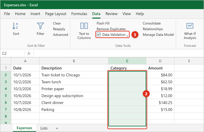
Go to the sheet where people will enter data and select the cell, or the whole range of cells, that should show the arrow. For example, select C2:C50 to add the list to every row of a Category column at once. You can also select a single cell and copy it to other cells afterward.

Step 3: Open Data > Data Validation

Click the Data tab on the ribbon. In the Data Tools group, click Data Validation. If you click the small arrow on the button instead of the button itself, a short menu opens; choose Data Validation from it. The Data Validation dialog box opens on the Settings tab. If the button is grey and won’t respond, jump to Troubleshooting.

Step 4: Set Allow to List

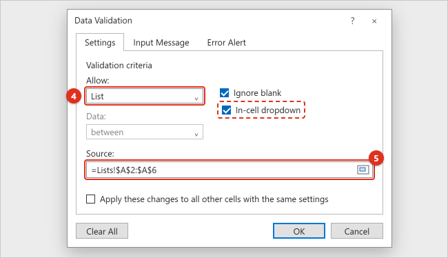
Under Validation criteria, open the Allow box (it says Any value by default) and choose List. Two checkboxes and a Source box appear. Leave In-cell dropdown checked; that’s the setting that shows the arrow. Leave Ignore blank checked if it’s OK for people to leave the cell empty.

Step 5: Select your list in the Source box

Click inside the Source box, then select the cells that hold your choices with the mouse. Don’t include the header. You can click another sheet’s tab while the box is active, so a list on a Lists sheet works fine. Excel fills in an absolute reference such as =Lists!$A$2:$A$6. The dollar signs matter: they keep every cell in your selection pointing at the same list. If you type the reference yourself, include them.

Step 6: Add an input message (optional)

Click the Input Message tab if you want a short note to pop up when someone selects the cell, such as “Pick a category from the list.” Check Show input message when cell is selected, then type a title and message. Microsoft lists a limit of 225 characters for the message. Skip this tab if you don’t want a pop-up.

Step 7: Choose what happens with typed entries (optional)

Click the Error Alert tab. With Show error alert after invalid data is entered checked and Style set to Stop (the default), Excel refuses anything typed into the cell that isn’t on the list. Choose Warning or Information to allow other entries after a message, or clear the checkbox to allow any entry silently. The messages section explains each style.

Step 8: Click OK

Click OK to close the dialog box. Nothing looks different yet, because Excel only shows the arrow on the cell that’s currently selected.

Step 9: Test the drop-down

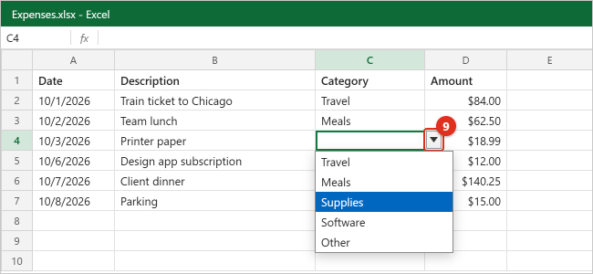
Click one of the cells you set up. A small arrow appears at the right edge of the cell. Click it, or press Alt+Down Arrow, and pick an item. The item fills the cell. Then try typing something that isn’t on the list and press Enter to make sure the error alert behaves the way you want. If some entries look cut off, widen the column; the list is only as wide as the cell.

Worked example: an expense log with a Category list

Suppose you track expenses on a sheet named Expenses, and people keep typing “Meal”, “meals”, and “Food” for the same thing. A drop-down list fixes that. Here is the setup.

On a second sheet named Lists, type the categories in column A:

Cell	Lists sheet, column A
A1	Categories (header, not part of the list)
A2	Travel
A3	Meals
A4	Supplies
A5	Software
A6	Other

On the Expenses sheet, the data looks like this, with column C getting the drop-down:

	A: Date	B: Description	C: Category	D: Amount
2	10/1/2026	Train ticket to Chicago	Travel	$84.00
3	10/2/2026	Team lunch	Meals	$62.50
4	10/3/2026	Printer paper	(pick from list)	$18.99
5	10/6/2026	Design app subscription	(pick from list)	$12.00

Select C2:C200 on the Expenses sheet, open Data > Data Validation, set Allow to List, click in Source, click the Lists tab, select A2:A6, and click OK. The Source box reads =Lists!$A$2:$A$6. Every Category cell from row 2 to row 200 now offers the same five choices, and with the Stop style left on, typing “Food” is refused.

Why use 200 rows instead of only the rows you have? It means new expenses typed below the current data already have the drop-down. If you format the expense data itself as a table and apply the rule to the whole Category column of that table, Excel normally carries the rule down to new rows as the table grows.

The values already in C2 and C3 stay as they are when you add the rule. Data validation doesn’t check or change existing entries. To find any old entries that aren’t on the list, use Data > Data Validation (click the arrow on the button) > Circle Invalid Data, as described in Troubleshooting.

Type the items directly into the Source box

For a short, fixed set of choices, you don’t need cells at all.

1. Select the cells that should get the drop-down.
2. Go to Data > Data Validation and set Allow to List.
3. In Source, type the choices separated by commas with no spaces, such as Yes,No,Maybe or Low,Medium,High. Don’t start with an equal sign.
4. Click OK.

Each item appears on its own line in the drop-down, in the order you typed it. Keep these limitations in mind:

• Changing it means reopening the dialog. There’s no list on the sheet to edit, so this is best for choices like Yes/No that won’t change.
• Your list separator might be a semicolon. On computers where Windows uses a comma as the decimal symbol (common in much of Europe), Excel expects Yes;No;Maybe instead. If your whole entry shows up as one item, try semicolons.
• Items can’t contain the separator. A choice like “Smith, John” would be split into two items. Put such items in cells instead.
• There’s a length limit. The Source box only holds a limited number of characters (commonly cited as 255). For long lists, use cells.

Make the list update automatically with an Excel table

A drop-down based on a plain range such as =$A$2:$A$6 doesn’t notice an item typed in A7. An Excel table fixes that, because a table expands when you type directly below it, and drop-downs based on the table follow along. This works in every Windows version covered here, with no formulas.

Step 1: Turn the list into a table

Click any item in your list and press Ctrl+T (or go to Insert > Table). In the Create Table dialog box, make sure the range is right and that My table has headers is checked if your list has a header, then click OK. The list gets banded formatting and a filter button in the header.

Step 2: Give the table a clear name (optional)

With a cell in the table selected, open the Table Design tab (called Table on some versions) and type a name such as tblCategories in the Table Name box. This helps if you later use the name approach below.

Step 3: Point the drop-down at the table’s data cells

Select the cells that need the drop-down, open Data > Data Validation, set Allow to List, click in Source, and drag over the table’s data cells (not the header). Excel shows a normal-looking reference such as =Lists!$A$2:$A$6. Click OK.

Step 4: Add an item and check the result

Type a new item, such as “Training”, in the first empty cell directly below the table and press Enter. The table expands to include it, and the drop-down now shows six choices. If you reopen the dialog box, you’ll see that the Source reference was extended to row 7 for you. Leave no blank row between the table and the new item, or the table won’t expand.

If you’d rather the Source box show the table by name, create a named range that refers to the table column (next section) and use that name as the source. Excel doesn’t always accept a table reference such as tblCategories[Categories] typed straight into the Source box. If it refuses, either use a name or wrap the reference in INDIRECT, like =INDIRECT("tblCategories[Categories]").

Use a named range or a list on another sheet

A named range is a label, such as Categories, that stands for a group of cells. Using a name as the source makes the rule easier to read, and it’s handy when several drop-downs share one list.

Step 1: Name the list

Select the list items (without the header). Click the Name Box to the left of the formula bar, type a name with no spaces, such as Categories, and press Enter. You can also use Formulas > Define Name, which lets you type a comment and confirm the scope is Workbook.

Step 2: Use the name as the source

Select the cells for the drop-down, open Data > Data Validation, set Allow to List, and type =Categories in Source. If you forget the name, press F3 while the cursor is in the Source box to pick it from a list. Click OK.

Step 3: Make the name grow (optional)

A name pointing at fixed cells doesn’t grow by itself. To get the automatic behavior, open Formulas > Name Manager, select the name, and change Refers to so it points at a table column, such as =tblCategories[Categories], then click the checkmark and Close. Every drop-down using =Categories now follows the table.

Hiding the list sheet. Once the drop-down works, you can right-click the Lists sheet tab and choose Hide. The drop-downs keep working. To stop people from unhiding or changing the list, protect the workbook structure with Review > Protect Workbook. Microsoft’s guide to locking specific areas of a protected worksheet explains the protection options.

Build the list with a formula

The Source box accepts any formula that returns a range, which opens up a few useful tricks.

A sorted list with no duplicates (Microsoft 365, Excel 2024, Excel 2021)

If your choices are buried in a column that repeats values, such as a column of vendor names in an order log, you can build a clean list with a dynamic array formula and point the drop-down at its results.

1. In an empty cell with plenty of empty cells below it, such as H2, enter =SORT(UNIQUE(B2:B500)). Excel “spills” the results down the column, one vendor per cell, sorted A to Z.
2. Select the cells for the drop-down and open Data > Data Validation with Allow set to List.
3. In Source, type =$H$2# and click OK.

The # after the cell address is the spill range operator. It means “every cell the formula in H2 returns,” so the drop-down grows and shrinks with the results. Put the formula in a cell rather than in the Source box; data validation doesn’t accept these functions typed directly into Source. If the column you’re summarizing contains blank cells, UNIQUE returns a 0 for them; use =SORT(UNIQUE(FILTER(B2:B500,B2:B500<>""))) to leave blanks out. If something blocks the cells below H2, the formula shows #SPILL! and the drop-down stops working until you clear the way.

A growing list without a table (Excel 2019 and 2016)

Older versions without dynamic arrays can use OFFSET and COUNTA in the Source box. For a list that starts in A2 of the Lists sheet with a header in A1:

=OFFSET(Lists!$A$2,0,0,COUNTA(Lists!$A:$A)-1,1)

COUNTA counts the filled cells in column A, the -1 removes the header from the count, and OFFSET returns a range that many rows tall starting at A2. The list must not contain blank cells, or the last item drops off. A table is easier when it’s available, and it’s available in every version covered here, so treat this as an option for workbooks that can’t use tables.

Trimming empty cells (Microsoft 365 only)

Current Microsoft 365 builds include the TRIMRANGE function and “trim references”, which let a large range such as $A$2:.$A$200 (note the period after the colon) ignore the empty cells at the end. Microsoft documents these for formulas; if your build accepts one in the Source box, it gives you a growing list with no table. If Excel shows an error, use a table instead. Workbooks that use trim references won’t behave the same when opened in Excel 2024 or earlier.

Create a dependent (cascading) drop-down list

A dependent drop-down is a second list whose choices change based on what was picked in the first one. For example, pick “Office” in a Department column and the Item column offers only office items; pick “Kitchen” and it offers kitchen items.

Method A: INDIRECT with named ranges (all versions)

Start by laying out each group of choices in its own column on the Lists sheet, with the first-list choice as the header:

	D: Office	E: Kitchen	F: Cleaning
2	Printer paper	Coffee	Paper towels
3	Pens	Cups	Trash bags
4	Sticky notes	Dish soap	Disinfectant

1. Create one name per column. Select D1:F4, go to Formulas > Create from Selection, check only Top row, and click OK. Excel creates the names Office, Kitchen, and Cleaning, each pointing to the three items under that header. Header text with spaces becomes a name with underscores, so “Break Room” becomes Break_Room.
2. Make the first drop-down. On your data sheet, select the Department cells (say A2:A100), open Data > Data Validation, choose List, and enter =Lists!$D$1:$F$1 as the source, which lists the three headers.
3. Make the second drop-down. Select the Item cells (B2:B100) with B2 as the active cell, open Data > Data Validation, choose List, and enter =INDIRECT(A2) as the source. Use A2 without dollar signs so each row looks at its own Department cell. Excel may warn that “The Source currently evaluates to an error” because A2 is empty; click Yes to continue.
4. Test it. Pick “Kitchen” in A2, then open the arrow in B2. You should see Coffee, Cups, and Dish soap.

If some first-list choices contain spaces, use =INDIRECT(SUBSTITUTE(A2," ","_")) so “Break Room” finds the name Break_Room.

Method B: FILTER (Microsoft 365, Excel 2024, Excel 2021)

If your items are stored in a two-column list (Department in one column, Item in the next) instead of side-by-side columns, the FILTER function can build the second list without any names. This works best for a single entry cell, like a form at the top of a sheet.

1. Make the first drop-down in B1 (Department) as usual.
2. In a helper cell, such as J2, enter =FILTER(Lists!$I$2:$I$50,Lists!$H$2:$H$50=$B$1), where column H holds departments and column I holds items. The matching items spill down from J2.
3. Give the second cell (B2) a drop-down with the source =$J$2#.

Whichever method you use, Excel doesn’t clear the second cell when someone changes the first. If a row says “Kitchen” and “Pens”, the old choice simply stays. Use Circle Invalid Data to spot mismatches, or ask people to pick the second value again after changing the first.

Add an input message and an error alert

The two other tabs in the Data Validation dialog box control what people see.

Input Message

An input message is a small yellow note that appears next to the cell when it’s selected. It’s useful for instructions such as “Choose the category that best matches the receipt.” Check Show input message when cell is selected, type a Title and an Input message, and click OK. Clear the checkbox later to turn it off without deleting the text.

Error Alert styles

The error alert decides what happens when someone types an entry that isn’t on the list. Picking from the arrow never triggers it.

Style	What the person sees	Can they keep an entry that isn’t on the list?
Stop	A message with Retry and Cancel	No. They must pick or type a listed value, or cancel.
Warning	A message asking “Continue?” with Yes, No, and Cancel	Yes, if they click Yes.
Information	A message with OK and Cancel	Yes, if they click OK.
Alert turned off	Nothing	Yes, always. The arrow is just a shortcut.

If you leave the title and message blank, Excel uses a generic title (“Microsoft Excel”) and a message saying the value doesn’t match the restrictions defined for the cell. A custom message such as “Choose a category from the list, or ask Alex to add a new one” is much friendlier. If people already see the default message and aren’t sure why, our guide to fixing the “This value doesn’t match the data validation restrictions” error walks through the common causes.

Use, copy, and find drop-down lists

Picking an item

• Mouse: select the cell and click the arrow at its right edge.
• Keyboard: select the cell and press Alt+Down Arrow, then use the arrow keys and Enter.
• Typing with AutoComplete: in current Microsoft 365 versions, typing a few letters in a drop-down cell narrows the list to matching items, and the match can be anywhere in the item, so typing “ware” finds “Software”. Older versions don’t filter the list this way.

Copying a drop-down to more cells

• Copy and paste: copy a cell that has the drop-down and paste it into other cells. This copies the rule along with the cell’s value and formatting.
• Paste only the drop-down: copy the cell, select the destination cells, press Ctrl+Alt+V (or Home > Paste > Paste Special), choose Validation, and click OK. The destination keeps its own values and formatting.
• Fill handle: dragging the small square at the bottom-right corner of the cell also copies the rule, but it copies the value too.

Be careful in the other direction: pasting an ordinary cell on top of a drop-down cell replaces its validation, and the arrow disappears without a warning. Pasted values also skip the validation check entirely, so a pasted “Food” is accepted even with the Stop style on.

Finding every cell that has a drop-down

The arrow only appears on the selected cell, so drop-downs are easy to lose track of. Go to Home > Find & Select > Data Validation to select every cell on the sheet that has a validation rule. For more control, use Home > Find & Select > Go To Special, choose Data validation, and pick All or Same (only cells with the same rule as the active cell). Giving those cells a fill color makes them easy to spot.

Edit, add, or remove items

How you change the choices depends on the source. Select a drop-down cell and open Data > Data Validation to see what the Source box contains.

• Typed items: edit the text in Source. Check Apply these changes to all other cells with the same settings so every matching drop-down updates, then click OK.
• A range of cells: change the items on the sheet. To add one in the middle, right-click an item, choose Insert > Shift cells down, and type the new item; Excel extends the reference for you. If you add items below the end of the range, reopen the dialog, reselect the full range in Source, and check Apply these changes to all other cells with the same settings.
• A table: type new items directly below the table. To remove one, delete it and, for an item in the middle, right-click and choose Delete > Table Rows so no gap is left.
• A named range: change the items, then fix the range in Formulas > Name Manager if needed.

Removing an item from the list doesn’t change cells where it was already chosen. Use Circle Invalid Data to find them.

To take the drop-down away completely while keeping the values in the cells, select the cells, open Data > Data Validation, click Clear All, and click OK. Our guide on how to remove a drop-down list in Excel covers this in detail, including what to do when Excel asks about extending the selection. And if you need people to pick more than one item per cell, a standard drop-down can’t do it; see how to select multiple items from a dropdown list in Excel for the macro-based workaround and its trade-offs.

Create a drop-down list in Excel for Mac

These steps are for Excel for Microsoft 365 for Mac, Excel 2024 for Mac, and Excel 2021 for Mac.

1. Type the list items in a single column or row with no blank cells. Press Command+T to make it a table if you want the list to grow automatically.
2. Select the cells where you want the drop-down.
3. On the Data tab, click Data Validation. On some versions and window sizes, the button is labeled Validate or shows only an icon; hover over the buttons in the tools area to find it.
4. On the Settings tab, open the Allow pop-up menu and choose List.
5. Click in the Source box and select your list on the sheet. The dialog box shrinks while you select; press Return or click the expand button to bring it back. You can also type comma-separated items, like Yes,No.
6. Use the Input Message and Error Alert tabs if you want them, then click OK.

On a Mac, select the cell and click the arrow to pick an item. The table, named range, formula, and dependent methods above work the same way; use Command wherever the Windows steps say Ctrl.

Create a drop-down list in Excel for the web

Excel for the web (in a browser at office.com or through OneDrive or SharePoint) can create and use drop-down lists without the desktop app.

1. Open the workbook in your browser and make sure you’re in editing mode (not Viewing).
2. Type your list items, ideally in a table (Insert > Table).
3. Select the cells that should get the drop-down.
4. Go to the Data tab and select Data Validation in the Data Tools group. On a narrow browser window, it may be inside a Data Tools button or the … overflow menu.
5. On the Settings tab, set Allow to List.
6. In Source, select the list cells (without the header) or type items separated by commas, such as Fruit,Vegetables,Grains.
7. Check Ignore blank if blank cells are OK, and keep In-cell dropdown checked.
8. Optionally use the Input Message tab (checkbox Show message) and the Error Alert tab (checkbox Show Alert and a Type box for Stop, Warning, or Information).
9. Select OK.

Drop-downs made in desktop Excel work in the browser, and the other way around. Form-control and ActiveX combo boxes (next section) don’t work in Excel for the web, which is a good reason to stick with data validation lists for shared workbooks.

Other kinds of drop-down: combo box controls

Data validation lists cover almost every need, but desktop Excel has two other drop-down objects. Both live on the Developer tab, which is hidden by default; our guide on how to show the Developer tab in Excel explains how to turn it on.

• Combo Box (Form Control): go to Developer > Insert > Combo Box (Form Control) and draw it on the sheet. Right-click it, choose Format Control, and set an Input range (the list) and a Cell link. The linked cell receives the position number of the chosen item (for example, 3 for the third item), so use =INDEX(list,linked_cell) to get the item text. It floats over the grid, can be resized, and doesn’t allow typed entries, which makes it popular on dashboards.
• Combo Box (ActiveX Control): more formatting options, but it requires Design Mode to edit and doesn’t work in Excel for Mac or Excel for the web. Avoid it unless you’re building a Windows-only tool.

Neither control is copied down a column the way a validation list is, so for row-by-row data entry, data validation is the better choice.

Troubleshooting

The Data Validation button is grey

• You’re still editing a cell. If the cursor is blinking inside a cell, press Enter or Esc first; the command is unavailable while you’re typing.
• The sheet is protected. Go to Review > Unprotect Sheet (you may need the password), add the drop-down, and protect the sheet again. Before protecting, unlock the drop-down cells (Home > Format > Format Cells > Protection, clear Locked) so people can still pick from them.
• The workbook uses the legacy Shared Workbook feature. Stop sharing it to change validation, then share it again. Co-authoring through OneDrive or SharePoint doesn’t have this restriction.
• Several sheets are grouped. If the title bar says “Group”, right-click a sheet tab and choose Ungroup Sheets.

The drop-down arrow doesn’t appear

• The arrow only shows on the selected cell. Click the cell itself.
• Open Data > Data Validation and make sure In-cell dropdown is checked. With it cleared, the rule still restricts typing but shows no arrow.
• Check that the validation is still there. A paste over the cell may have replaced it; use Home > Find & Select > Data Validation to see which cells still have rules.
• If arrows are missing in the whole workbook, check File > Options > Advanced, under Display options for this workbook, that For objects, show is set to All. Hiding objects can also hide drop-down arrows.

“The Source currently evaluates to an error”

Excel shows this when the source formula or reference can’t be read right now. For a dependent list, it usually just means the first cell is empty; click Yes and test after picking a value in the first list. Otherwise, check the name for typos (Name Manager lists them), make sure a referenced sheet hasn’t been renamed or deleted, and make sure a spill formula isn’t showing #SPILL!.

The list shows blank lines or the wrong items

• Blank lines: the source range includes empty cells. Shrink the range, use a table, or use a formula that filters out blanks.
• Each row shows a different list: the source reference is missing its dollar signs (for example, =E2:E6 instead of =$E$2:$E$6), so it shifted as it was applied to each row. Fix the reference and check Apply these changes to all other cells with the same settings.
• The whole typed list shows as one item: your system uses semicolons as the list separator. Replace the commas with semicolons.
• New items don’t appear: the source is a fixed range. Extend it, or switch to a table.

Entries that aren’t on the list got in anyway

Validation only checks values that are typed in. Pasted values, values entered before the rule existed, and values from formulas aren’t checked. Select the range and choose Data > Data Validation (click the arrow on the button) > Circle Invalid Data to draw red circles around anything that breaks the rule. Correct those cells, and the circles disappear; or use Clear Validation Circles from the same menu.

The text in the list is too small or cut off

The list’s width matches the column width, so widen the column to show long items. The font size of a data validation list can’t be changed separately; it follows the worksheet zoom, so zooming in makes the list easier to read. If you need a larger, styled control, use a form-control combo box instead.

How to undo a mistake

Press Ctrl+Z (Command+Z on a Mac) right after adding or changing a rule to reverse it. If the workbook is saved in OneDrive or SharePoint, File > Info > Version History lets you open an earlier version. Otherwise, reopen the dialog and click Clear All to start over.

Frequently Asked Questions

What’s the fastest way to add a Yes/No drop-down in Excel?

Select the cells, go to Data > Data Validation, set Allow to List, type Yes,No in Source, and click OK. No cells or formulas are needed for a two-choice list.

Can the list come from a different sheet?

Yes. While the cursor is in the Source box, click the other sheet’s tab and select the cells. Excel writes a reference like =Lists!$A$2:$A$6. You can hide that sheet afterward and the drop-down keeps working.

Can the list come from a different workbook?

It can, but it’s fragile: the drop-down only shows choices when the other workbook is available, and links break when files are moved or renamed. Copying the list into a hidden sheet in the same workbook is more reliable.

How do I make the drop-down list update automatically?

Put the items in an Excel table (select a cell in the list and press Ctrl+T) and select the table’s data cells as the source. When you type a new item directly below the table, the table and the drop-down both expand.

Can people select more than one item in a drop-down?

Not with a standard data validation list; each pick replaces the previous one. Keeping several choices in one cell needs a VBA macro in desktop Excel, which doesn’t run in Excel for the web. Using separate columns or one row per choice is usually easier to sort and count.

Why can I still type values that aren’t on the list?

Either the error alert is turned off or set to Warning or Information, which allow other entries. Open the Error Alert tab, check Show error alert after invalid data is entered, and set Style to Stop. Pasted values still bypass validation.

How do I change the order of the items?

The drop-down shows items in the same order as the source. Sort the source cells (Data > Sort A to Z), or rearrange them by hand. For typed items, retype them in the order you want. A SORT formula can also keep a list in order automatically.

Does a drop-down list work in Google Sheets?

Google Sheets has its own drop-down feature under Data > Data validation, and Excel drop-downs usually carry over when you open an Excel file there. For the Sheets steps, see how to create a Google Sheets drop-down menu.

Does deleting a cell’s value remove the drop-down?

No. Pressing Delete clears the value but leaves the rule and the arrow. To remove the drop-down itself, use Data > Data Validation > Clear All.

Next step

Start with a simple list on its own sheet, turn it into a table, and point your drop-down at it. That setup handles new items on its own and is the easiest to hand off to coworkers. Once it’s working, add a friendly error message, and consider a dependent list if your choices fall into groups. Microsoft’s own Create a drop-down list page has the Windows, Mac, and web steps side by side if you want a quick reference.