How to Make a Graph in Google Sheets

You have a table of numbers due in a report or a meeting, and you are not sure which picture will make the point. In Google Sheets, Insert > Chart builds a chart from the cells you select, and the Setup tab of the Chart editor switches its type at any time, so a first choice is never final. The more useful decision is which question your data answers, so start there.

Pick the graph type by the question you are answering

The words “graph” and “chart” mean the same thing here; Sheets uses “chart” in its menus. Google’s chart types page describes what each one is for. This table turns those descriptions into the questions people actually bring to a meeting.

The question you want to answer	Chart type to try first	Why it fits
How did this change over time?	Line	Google’s stated use for it is trends or data over a time period
How do these groups compare?	Column	Shows categories of data, especially when each has subcategories
How far apart are these items?	Bar	Shows the difference between data points, and long names read easily along a side axis
What share of the whole does each part hold?	Pie or doughnut	Shows proportions of a whole; best kept to a few slices
Do two measurements move together?	Scatter	Plots two numeric variables against each other to show a pattern
How are my values spread out?	Histogram	Shows the distribution of a data set across buckets
Can I show one series as columns and another as a line?	Combo	Shows each data series as a different marker type
What added to or subtracted from a starting figure?	Waterfall	Shows how later values add to or take away from a start value

Variants live alongside these in the same list: stacked and 100% stacked versions of area, column and bar charts, plus doughnut under pie and bubble under scatter. Google also lists Stock, Organizational, Tree map, Geo, Radar, Gauge, Annotated timeline, Box & whisker and Table charts for more specialized jobs.

If your question is about distribution, making a histogram in Google Sheets needs a little more explanation than this article has room for. If you are testing whether two columns are related, pair a scatter chart with a correlation calculation so you have a number to go with the picture.

Build a graph from a monthly sales table

A worked example makes the editor easier to follow. Suppose the question is “how did two products sell over six months?” That is a change-over-time question, so a line chart is the first try. These figures are invented for the example:

Month	Product A	Product B
Jan	120	80
Feb	135	95
Mar	128	110
Apr	150	125
May	162	140
Jun	170	165

1. Type the table into a sheet with Month in cell A1, so the labels sit in the first column and the names sit in the first row. Leave out blank rows so the example stays simple.
2. Highlight the table from A1 to C7, taking in the top row of names.
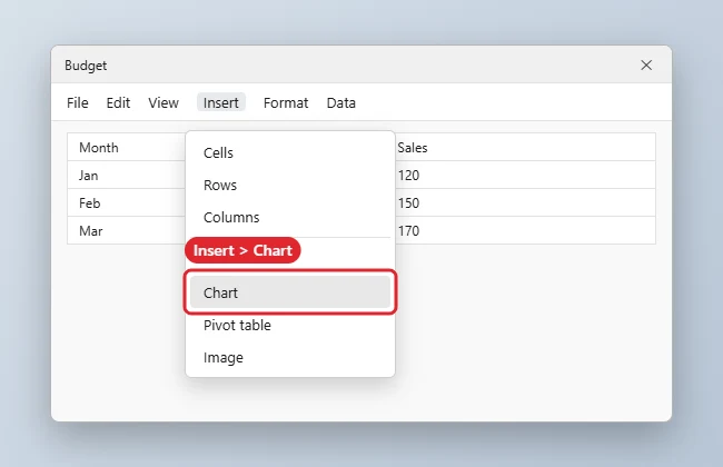
3. Click Insert, then Chart. Sheets draws a first version and opens the Chart editor at the right side of the window.

4. In the editor, click Setup. Under Chart type, open the dropdown and pick a line chart. The first version Sheets draws may be a different type, so make this choice yourself.
5. Look at Data range and confirm it reads A1:C7.
6. Click Customize, open Chart & axis title, and type a title that states the finding, such as “Product B nearly caught Product A by June.”

The goal is two lines, one for each product, with the months running along the bottom and the product names in the legend. If what you see is different, the section on fixing a graph below covers the usual causes. If you close the editor, double-click the chart to bring it back.

The same steps work with most tables. If you have raw text instead of numbers, such as a list of survey answers, tally it first with a count of how many times each word appears and graph the counts. Tidier source data also helps, and converting a range to a table is one way to get there.

Fix a graph that looks wrong

When a first draft looks odd, a setting or two often corrects it. Find your symptom here.

What you see	Likely cause	Fix
Only one line or set of columns appears	The range is too narrow	Double-click the chart, click Setup, click the grid icon under Data range, select all the cells, then click OK
The cells you need are in another part of the sheet	They are not next to the rest	In the same box, use Add another range, then click OK
Your header row is plotted as a value, or the legend shows no names	Sheets is not using it as a header	In Setup, select Use row N as headers, with N being your header row
Months are drawn as lines and products run along the bottom	Rows and columns are read the wrong way round	In Setup, select Switch rows / columns, and Use column N as headers if needed
The picture is right but hard to read	The type does not fit the question	Go back to Chart type and try the suggestion from the first table
A title or legend landed in an awkward spot	It was moved	Right-click it and click Reset layout. To reset everything, go to Customize, then Chart style, then Reset layout

If none of those fit, inspect the source cells. A blank row inside the range or a number stored as text is worth ruling out, since either one could change how the data gets plotted. Google’s page does not list these as causes, so treat them as things to check rather than as a sure diagnosis.

What Setup controls and what Customize controls

The Chart editor has two tabs, and most confusion comes from looking in the wrong one. As a rule of thumb, Setup decides what is being graphed and Customize decides how it looks. Labels below come from Google’s help page on charts.

You want to change	Tab	Where to look
The kind of graph	Setup	Chart type
Which cells are included	Setup	Data range, using the grid icon
Cells from somewhere else	Setup	Data range, then Add another range
Which row or column supplies the names	Setup	Use row N as headers or Use column N as headers (N is the row or column number)
Which way the table is read	Setup	Switch rows / columns
Background and fonts	Customize	Chart style
Titles on the chart and axes	Customize	Chart & axis title
The key that names each series	Customize	Legend
The background lines	Customize	Gridlines

Make it readable before anyone else sees it

A graph for a meeting has seconds to get its point across. A few changes do most of that work:

• Write a title that says something. “Sales by month” labels the chart. “Product B nearly caught Product A by June” tells people what to see. Use Chart & axis title, and add axis titles when units are not obvious.
• Trim the key. If there is only one series, the title can do the legend’s job. Google lets you delete a specific item by double-clicking it and pressing Delete or Backspace, which works for items such as titles and legends.
• Quiet the background. Reduce Gridlines to what people need in order to read values.
• Point at the one bar that matters. Right-click a bar or point, then click Format Data Point to set it apart. Google notes that you can add borders to bars and columns, though not to points or lines. For a full color scheme, see changing chart colors in Google Sheets.
• Place it with care. Click the chart and drag it to move it, then drag the blue markers to resize it. Avoid covering the numbers beneath it.

Get the graph out of Sheets

How you share the graph depends on where your audience will see it, so match the route to the destination.

Destination	Route
A picture in an email or a printed handout	Download as PNG, PDF or SVG
A web page or a link people can open	Publish chart
A Docs report or Slides deck	Insert > Chart > From Sheets

Download an image or PDF

1. Click the chart.
2. At the top right of the chart, click the More icon, then Download as.
3. Choose SVG, PNG or PDF, as listed on Google’s save or publish page.

A dedicated walk-through is in downloading a Google Sheets chart as a PNG.

Publish a link or embed code

Before you publish, confirm the figures are fine for whoever could end up with the link. Then:

1. Click the chart, then the More icon at its top right.
2. Click Publish chart.
3. Choose Link to copy and share a link, or Embed to copy HTML code for a website or blog.
4. Click Publish.

Bring it into Docs or Slides

Google’s linking help page has a detail worth knowing first: people with access to your document or presentation can view linked charts even if they cannot open the spreadsheet. Check that nothing in the chart should stay private.

1. In the document or presentation, click Insert > Chart > From Sheets.
2. Click the spreadsheet, then Select.
3. Click the chart you want.
4. Leave Link to spreadsheet checked for a chart you can refresh, or uncheck it for a fixed copy.
5. Click Import.

To refresh a linked chart, click Update at its top right corner. For several at once, go to Tools > Linked objects and click Update all at the bottom. More on the Slides side is in inserting a Google Sheet into Google Slides, and the Docs version covers tables too.

Build one on a phone or tablet

Google documents the same short path for the Android and iPhone and iPad apps:

1. Open the spreadsheet in the Google Sheets app.
2. Select the cells you want in the chart.
3. Tap Insert (the plus icon on Android), then Chart.
4. Tap Type if you want a different chart, then choose one.
5. Tap Done.

To change it later, double-tap the chart and tap Edit chart, where you can change the Type, Legend, Titles and Color. Tap and drag the chart to move it, or use the blue markers to resize it.

This is enough for a quick look. The labels described above come from the computer version, so plan on a browser for detailed editing or to use the download and publish steps Google documents for computers.

Sheets chart questions

Which download format should I pick?

Google lists the three formats but does not say which to use, so treat this as general guidance. PNG is the easy choice for email and most slide software, since it is an ordinary image. SVG is a scalable format that suits design tools and web pages. PDF is handy for a page you plan to print or attach as a document.

If I edit a linked chart inside Slides, does the spreadsheet change?

No. Google says edits to a linked object in your new file are not copied back to the original. It also warns that changes in the original override those edits when you update the link, so make lasting changes in the spreadsheet.

Can two series use different scales?

Yes, on some charts. Google’s axis help page says you can add a second Y-axis to a line, area or column chart: double-click the chart, click Customize, click Series, choose the series next to Apply to, then choose Right axis under Axis. That section does not mention combo charts.

A good next step: copy your real table into a blank tab, run through the first table to choose a type, and build it. Trying two chart types and comparing them side by side usually settles the question.