How to Use the QUERY Function in Google Sheets

To use the QUERY function in Google Sheets, click an empty cell and type =QUERY(range, "query", 1), for example =QUERY(A1:F11, "select B, F where F > 1000", 1), then press Enter. The first argument is your data, the second is a short instruction written in quotation marks that says which columns to show and which rows to keep, and the 1 tells Sheets your data has one header row. The results spill into the cells below and to the right, and they update on their own whenever the source data changes.

QUERY can do the jobs of several tools at once: it filters like a filter, sorts like Sort range, totals like a pivot table, and picks columns like a lookup. This guide explains the syntax in plain terms, walks through a first formula step by step, and then covers every clause you are likely to need, plus text, number, and date conditions, cell references, combining tabs and files, and fixes for the error messages people hit most.

What you need and what this covers

• Google Sheets on the web in a browser on a computer. QUERY is a built-in function, so there is nothing to install or turn on. It works the same in free Google accounts and Google Workspace accounts.
• A table of data with one header row and one kind of value per column (for example, dates in one column and numbers in another).
• Phones and tablets: the Google Sheets app for Android and iPhone calculates QUERY formulas that already exist, and you can type new ones, but long query strings are much easier to write and check on a computer.
• Excel users: Microsoft Excel does not have a QUERY worksheet function. If you open a Sheets file in Excel, these formulas will not work there. In Excel, the closest tools are FILTER, SORT, and Power Query.

The steps and examples below reflect Google Sheets on the web as of October 2026 and Google’s own documentation for the QUERY function and the query language it uses.

QUERY syntax explained

The function has three parts:

=QUERY(data, query, [headers])

• data (required): the cells to search, such as A1:F11, an open-ended range such as A1:F, a range on another tab such as Orders!A1:F, or the result of another function such as IMPORTRANGE.
• query (required): the instructions, written in Google’s query language and wrapped in double quotation marks. You can also type the instructions in a cell and point to that cell instead.
• headers (optional): how many header rows sit at the top of your data. If you leave it out, or use -1, Sheets guesses from the content. Typing 1 (or 0 when there are no headers) avoids surprises, so the examples in this guide always include it.

The query language is a simplified relative of SQL, the language used to ask databases for information. You do not need to know SQL. A query is made of short clauses (keywords followed by details), such as select B, F (show columns B and F) and where F > 1000 (keep only rows where column F is more than 1,000). Keywords such as select and where are not case-sensitive, so SELECT and select both work.

Two rules trip up nearly every beginner, so they are worth knowing before you start:

• Columns are named by letter, not by header text. With a normal range, B means column B of the sheet. You cannot write select Revenue. (Data built from curly braces or IMPORTRANGE uses Col1, Col2 instead; that is covered below.)
• Text goes in single quotes inside the query. The whole query sits in double quotes, so a text value inside it uses single quotes: "select * where C = 'East'". Numbers need no quotes at all.

The sample data used in this guide

Every example uses this small sales table on a tab named Orders, in cells A1:F11. You can type it into a blank spreadsheet to follow along. Put the formulas on a second tab (this guide calls it Report) so the results have empty space to spill into.

Row	A: Date	B: Rep	C: Region	D: Product	E: Units	F: Revenue
2	1/5/2026	Alex Rivera	East	Laptop	2	1800
3	1/9/2026	Jordan Lee	West	Monitor	5	1250
4	1/14/2026	Priya Shah	East	Keyboard	10	450
5	1/20/2026	Sam Ortiz	South	Laptop	1	900
6	2/2/2026	Alex Rivera	East	Monitor	3	750
7	2/11/2026	Jordan Lee	West	Laptop	3	2700
8	2/17/2026	Priya Shah	South	Keyboard	8	360
9	2/25/2026	Sam Ortiz	West	Monitor	4	1000
10	3/3/2026	Alex Rivera	East	Laptop	1	900
11	3/12/2026	Priya Shah	East	Monitor	2	500

Make sure the Date column holds real dates, not text that only looks like dates. A quick test: in an empty cell, type =ISNUMBER(A2). Sheets stores real dates as numbers, so TRUE means a real date and FALSE means text that only looks like one. Text dates are also usually left-aligned, while real dates line up on the right.

How to write your first QUERY formula

This first formula lists the rep, product, and revenue for every sale over $1,000.

Step 1: Click an empty cell with room below it

Go to the Report tab and click cell A1. QUERY returns a whole table, so the cells below and to the right must be empty. If anything is in the way, you will see a #REF! error instead of results.

Step 2: Type the function name and the data range

Type =QUERY( and then the range, including the header row: Orders!A1:F11. The tab name followed by an exclamation point tells Sheets the data is on another tab. If a tab name has spaces, wrap it in single quotes, for example 'Sales Data'!A1:F11. Type a comma after the range.

Step 3: Type the query in double quotes

Type "select B, D, F where F > 1000". This says: show columns B (Rep), D (Product), and F (Revenue), and keep only rows where column F is greater than 1000. Do not type a dollar sign or comma inside the number. Type another comma.

Step 4: Set the header count and press Enter

Type 1) to tell Sheets the data has one header row, so the full formula reads =QUERY(Orders!A1:F11, "select B, D, F where F > 1000", 1). Press Enter.

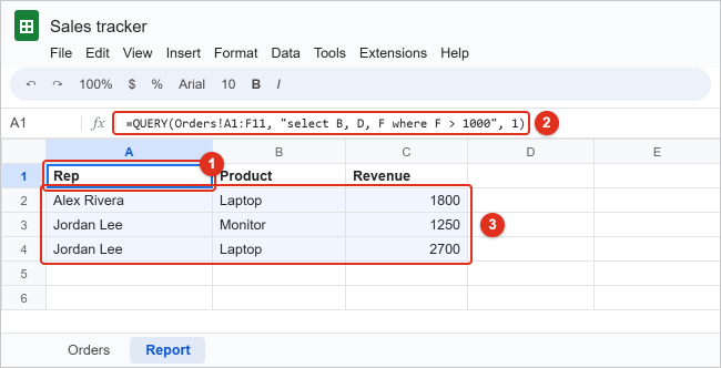
Step 5: Check the result

You should see a header row (Rep, Product, Revenue) and three sales: Alex Rivera’s $1,800 laptop, Jordan Lee’s $1,250 monitors, and Jordan Lee’s $2,700 laptops. Sam Ortiz’s $1,000 sale is not included because the condition is “greater than,” not “greater than or equal to.” Change > to >= to include it.

Only cell A1 contains a formula. The other cells show results that QUERY “spilled” into them, so you cannot edit them one by one. To change the output, edit the formula in A1. To remove the whole result, click A1 and press Delete. Your original data on the Orders tab is never changed by QUERY.

Step 6: Make the range grow with your data (optional)

Change Orders!A1:F11 to Orders!A1:F (no ending row number) so new rows added at the bottom are included automatically. With an open-ended range, add A is not null to your conditions when you group or count, so the empty rows at the bottom of the sheet do not appear as a blank group. For example: "select C, sum(F) where A is not null group by C".

Every QUERY clause and the order to use it in

You can combine as many clauses as you need in one query, but they must appear in this order. Putting them out of order (for example, ORDER BY before WHERE) causes a parse error.

Order	Clause	What it does	Example
1	select	Chooses which columns to show and in what order. select * (or no select) shows all columns.	select B, F
2	where	Keeps only the rows that meet a condition.	where C = 'East'
3	group by	Combines rows that share a value and calculates a total, count, or average for each group.	group by C
4	pivot	Turns each distinct value in a column into its own result column, like a pivot table.	pivot D
5	order by	Sorts the results. Add desc for largest first; asc is the default.	order by F desc
6	limit	Returns no more than the number of rows you name.	limit 3
7	offset	Skips the first rows of the result. It is applied before limit.	offset 3
8	label	Renames result column headers.	label F 'Sales'
9	format	Changes how numbers or dates are displayed in the result.	format F '$#,##0'
10	options	Rarely needed advanced settings, such as no_format.	options no_format

A memory aid for the first five: Select, Where, Group, Pivot, Order.

select: pick and reorder columns

=QUERY(Orders!A1:F11, "select D, B", 1) shows Product first and Rep second, even though they are in the opposite order on the Orders tab. You can also calculate new values in select. =QUERY(Orders!A1:F11, "select D, F / E label F / E 'Price per unit'", 1) divides revenue by units for each row and names the new column “Price per unit.” The query language supports +, -, *, and / on numbers.

order by and limit: sort and keep the top results

=QUERY(Orders!A1:F11, "select B, D, F order by F desc limit 3", 1) returns the three biggest sales: Jordan Lee’s $2,700 laptops, Alex Rivera’s $1,800 laptops, and Jordan Lee’s $1,250 monitors. To sort by more than one column, separate them with commas: order by C, F desc sorts by region A to Z, then by revenue from largest to smallest within each region.

offset: page through results

"select B, F order by F desc limit 3 offset 3" skips the top three sales and returns the next three. This is handy for building a “page 2” of a leaderboard.

format: control number display

QUERY results do not copy the formatting of your source cells, so currency often appears as plain numbers. Add a format clause such as format F '$#,##0' to show dollar signs and thousands separators, or format A 'MMM d, yyyy' for dates. You can also select the result cells and use Format > Number instead; that formatting stays as long as the result shape does not change.

Filtering rows with WHERE: text, numbers, and blanks

WHERE is the clause you will use most. These are the operators it understands.

Goal	Operator	Example query	Rows returned from the sample
Exact text match	=	select * where C = 'East'	5 East sales
Not equal	!= or <>	select * where D != 'Laptop'	6 non-laptop sales
Number comparison	>, <, >=, <=	select * where E >= 5	3 sales of 5+ units
Text anywhere in the cell	contains	select * where B contains 'Lee'	Jordan Lee’s 2 sales
Text at the start or end	starts with, ends with	select * where D starts with 'Key'	2 keyboard sales
Wildcard pattern	like (% = any characters, _ = one character)	select * where B like 'P%'	Priya Shah’s 3 sales
Regular expression	matches	select * where D matches 'Laptop|Monitor'	8 laptop or monitor sales
Empty or filled cells	is null, is not null	select * where F is not null	All 10 rows (none are blank)

Combine conditions with and, or, and not

Use and when every condition must be true and or when any one is enough. "select * where C = 'East' and F >= 900" returns Alex Rivera’s two East laptop sales ($1,800 and $900). "select * where C = 'West' or C = 'South'" returns all five West and South sales.

When you mix and with or, add parentheses so Sheets checks them in the order you mean: "select * where (C = 'West' or C = 'South') and D = 'Laptop'" returns only the two laptop sales from those regions. Use not to reverse a test, such as where not B contains 'Lee'.

Text matching is case-sensitive

The query language treats text and column identifiers as case-sensitive, so where C = 'east' finds nothing when your cells say “East.” To match regardless of capitalization, convert the column with lower() or upper() first and compare against lowercase or uppercase text: "select * where lower(C) = 'east'". Extra spaces also break exact matches. If a value looks right but does not match, check the source cells for a trailing space, or switch to contains.

One data type per column

Google’s documentation notes that each column in QUERY can hold only one type of value (text, number, true/false, or date/time). If a column mixes types, the most common type wins and the others are treated as empty. A Revenue column with a few cells that say “pending” will show those cells as blank in the result and leave them out of totals, with no error to warn you. Keep notes in a separate column, or convert the column so every cell has the same type.

Filtering and grouping by date

Dates are a common source of QUERY errors, because a date inside the query must be written in a fixed format with the word date in front of it: date 'yyyy-mm-dd'.

• After a date: "select * where A > date '2026-02-15'" returns the four sales from February 17 onward.
• Between two dates: "select * where A >= date '2026-02-01' and A < date '2026-03-01'" returns the four February sales, worth $4,810 in total. Using “less than March 1” is safer than “less than or equal to February 28” because it also works in leap years and with times.
• Dates with times: use datetime 'yyyy-mm-dd hh:mm:ss', for example datetime '2026-02-01 08:00:00'. For a time of day alone, use timeofday '08:00:00'.

If you write where A > '2/15/2026' without the date keyword, QUERY compares a date to a piece of text and returns either nothing or an error. If your column holds text instead of real dates, convert it first (for example, with DATEVALUE in a helper column) before querying.

Group sales by month

The query language has date functions, including year(), month(), day(), and quarter(). One catch: month() counts from 0, so January is 0 and December is 11. Add 1 to get normal month numbers:

=QUERY(Orders!A1:F11, "select month(A)+1, sum(F) group by month(A)+1 label month(A)+1 'Month', sum(F) 'Revenue'", 1)

The result shows month 1 with $4,400, month 2 with $4,810, and month 3 with $1,400. To group by year and month across several years, use group by year(A), month(A)+1 and select both.

Totals with GROUP BY, PIVOT, and LABEL

GROUP BY turns QUERY into a quick summary tool. It collects every row that shares a value and runs an aggregate function (a calculation across many rows) on each group. The five aggregate functions are sum(), avg(), count(), min(), and max(). Sum and avg work only on number columns; count, min, and max work on any type.

Total revenue by region

=QUERY(Orders!A1:F11, "select C, sum(F) group by C", 1) returns one row per region: East $4,400, South $1,260, and West $4,950. Without an ORDER BY, groups are listed alphabetically. The automatic header for the total is “sum Revenue.”

Sort the totals and rename the headers

To put the best region first and give the columns friendlier names, add order by and label:

=QUERY(Orders!A1:F11, "select C, sum(F) group by C order by sum(F) desc label C 'Region', sum(F) 'Total revenue'", 1)

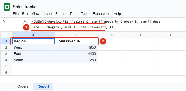
Notice that order by refers to sum(F), the calculated column, not to F. In label, list each column and its new name in single quotes, separated by commas.

The one rule GROUP BY enforces

Every column in select must either appear in group by or be inside an aggregate function. "select B, C, sum(F) group by C" fails because B (Rep) is neither grouped nor totaled. Fix it by grouping on both, group by B, C, which gives a total for each rep in each region, or by removing B.

Counts, averages, and several totals at once

=QUERY(Orders!A1:F11, "select B, count(F), sum(E), avg(F) group by B label count(F) 'Sales', sum(E) 'Units', avg(F) 'Average sale'", 1) returns one row per rep with the number of sales, units sold, and average sale value. Alex Rivera, for example, has 3 sales, 6 units, and an average sale of $1,150. Count skips empty cells, so count a column that is always filled in.

Cross-tab totals with PIVOT

PIVOT spreads one column’s values across the top of the result. =QUERY(Orders!A1:F11, "select C, sum(F) group by C pivot D", 1) gives one row per region and one column per product (Keyboard, Laptop, Monitor), with revenue in each cell. East shows $450, $2,700, and $1,250; South shows $360 and $900 with an empty Monitor cell because South sold no monitors; West shows an empty Keyboard cell, $2,700, and $2,250.

Two limits apply: the pivot column cannot also appear in select, group by, or order by, and when you use pivot, order by cannot sort by an aggregate such as sum(F). Without group by, pivot returns a single row of totals, for example "select sum(F) pivot C".

Using a cell value inside the query

Typing values straight into the query works, but a formula that reads its condition from a cell is easier to reuse. Because the query is just text, you build it by joining pieces with the ampersand (&) operator. Suppose cell H1 on the Report tab holds a region name:

• Text from a cell: =QUERY(Orders!A1:F11, "select B, D, F where C = '"&H1&"'", 1). Look closely at the quotes: a single quote, then a double quote to close the text, then &H1&, then a double quote to reopen the text, then a single quote. The single quotes end up around the region name.
• A number from a cell (say H2 holds 1000): "select * where F > "&H2. Numbers do not need single quotes.
• A date from a cell (say H3 holds a date): "select * where A >= date '"&TEXT(H3, "yyyy-mm-dd")&"'". TEXT converts the date into the exact format the query language expects.
• The whole query in a cell: type select B, F where F > 1000 into H4 (no outer double quotes) and use =QUERY(Orders!A1:F11, H4, 1).

Pair the text version with a dropdown list in H1 and you have a simple report that changes when someone picks a different region. Our guide to creating a Google Sheets drop-down menu shows how to add the list.

Col1 vs. column letters, multiple tabs, and IMPORTRANGE

When to use Col1, Col2, Col3

Column letters only work when the data argument is an ordinary range on a sheet. When the data is built by a formula, such as ranges stacked with curly braces or the result of IMPORTRANGE, the result has no sheet letters, so you refer to columns by position: Col1 is the first column of the data, Col2 the second, and so on. The capital C matters.

A tip that makes this easier: you can wrap a normal range in curly braces to switch it to Col notation on purpose, as in =QUERY({Orders!A1:F11}, "select Col2, Col6 where Col6 > 1000", 1). Because Col numbers count from the left edge of the data, the same query text works on a range that starts in any column. Note that neither letters nor Col numbers inside the quotes update if you later insert or delete columns, so recheck the query after changing the layout.

Query several tabs as one table

If January and February sales are on separate tabs with identical columns, stack them with curly braces and semicolons:

=QUERY({Jan!A2:F; Feb!A2:F}, "select Col2, sum(Col6) where Col1 is not null group by Col2", 0)

Three details make this work. Start each range at row 2 so header rows do not land in the middle of your data, set headers to 0 because the stacked data has no header row, and keep the same number of columns in every range or Sheets shows an error. The Col1 is not null condition drops the empty rows from the open-ended ranges. Use a comma instead of a semicolon inside the braces to place ranges side by side rather than on top of each other.

Query a different spreadsheet with IMPORTRANGE

IMPORTRANGE pulls a range from another Google Sheets file. Put it in the data position of QUERY and use Col notation:

=QUERY(IMPORTRANGE("https://docs.google.com/spreadsheets/d/your-file-id/edit", "Orders!A1:F"), "select Col2, Col6 where Col3 = 'West'", 1)

The first time a file pulls from a new source, you must approve the connection. The cell shows #REF!; point to it or click it and choose Allow Access.

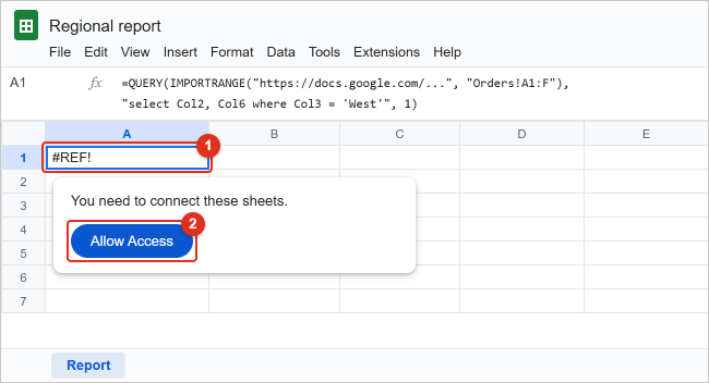
Before you allow access, know what it means: Google’s help notes that once access is granted, anyone who can edit the destination file can use IMPORTRANGE to pull any part of the source file. You need at least view access to the source; if you do not have it, open the source link and request access from the owner. Google also caps each import at about 10 MB of data, and imports refresh roughly every hour while the file is open, so querying a huge source can be slow. For a step-by-step look at IMPORTRANGE on its own, see how to pull data from another sheet in Google Sheets.

QUERY vs. FILTER, pivot tables, and VLOOKUP

QUERY is not always the best tool. Use this as a quick guide:

Task	Best choice	Why
Show rows that meet a condition, all columns	FILTER or QUERY	FILTER is shorter to write; QUERY is easier to extend later.
Show only some columns, sorted, from filtered rows	QUERY	One formula does select, where, and order by together.
Totals, counts, or averages by group in a formula	QUERY	GROUP BY and PIVOT do this without helper columns.
Interactive summary you can drag fields around in	Pivot table	Insert > Pivot table gives a point-and-click editor.
Return one matching value for each row	VLOOKUP or XLOOKUP	Lookups return a single value; QUERY returns a table.
Hide rows on the original data without a formula	A filter or filter view	Data > Create a filter changes what you see, not where data lives.

If you only need matching rows, the FILTER function is covered in our guide to filtering columns in Google Sheets. For single-value lookups, see how to use VLOOKUP in Google Sheets.

QUERY errors and how to fix them

Point to a cell with a red triangle in its corner to read the full error message. The wording below describes what you are likely to see; the exact text can vary slightly.

“Unable to parse query string for Function QUERY parameter 2”

Sheets could not understand the query text. Check these causes in order:

• Text values without single quotes, such as where C = East. It should be where C = 'East'.
• Clauses in the wrong order, such as order by before where. Use the order in the clause table.
• A typo in a keyword (selet, gruop by) or a missing comma between columns in select.
• Curly “smart” quotes pasted from a web page or document. Retype the quote marks in Sheets.
• Column letters used with curly-brace or IMPORTRANGE data. Switch to Col1, Col2.
• A date written without the date keyword or not in yyyy-mm-dd order.

“NO_COLUMN” message

The query names a column that is outside the data range, for example select G when the range is A1:F11. Expand the range or correct the letter. With Col notation, the number is higher than the number of columns in the data.

Message mentioning “ADD_COL_TO_GROUP_BY_OR_AGG”

A column in select is not in group by and not inside an aggregate function. Add it to group by or wrap it in sum(), count(), or another aggregate.

#N/A: “Query completed with an empty output”

The formula is valid but no rows matched. Check for a case mismatch, an extra space, or a number stored as text. To show a friendly message instead, wrap the formula: =IFERROR(QUERY(Orders!A1:F11, "select * where C = 'North'", 1), "No matching sales"). Be aware that IFERROR also hides real mistakes, so add it only after the formula works.

#REF!: “Array result was not expanded because it would overwrite data”

Something is in the cells where the result needs to spill. Clear those cells, or move the formula to a spot with more empty space. The message names the cell that is in the way.

#VALUE! or an error about sum or avg

Sum and avg only work on number columns. If the column you are totaling holds numbers stored as text (often from imported or pasted data), convert them with Format > Number > Number, or use VALUE in a helper column.

Some cells are blank, but there is no error

The column mixes data types, so the minority type is treated as empty. Clean up the column so every cell holds the same kind of value.

The header row shows up as a data row, or the first data row becomes a header

The headers argument is wrong or missing. Set it to the number of header rows in your range: 1 for one header row, 0 if your range starts below the headers. If you stacked ranges with curly braces, use 0.

The formula shows an error about the separator

Some spreadsheet locales use a comma as the decimal mark and expect semicolons between function arguments, as in =QUERY(A1:F11; "select *"; 1). Commas inside the query string itself stay as they are. You can check your locale in File > Settings.

A good debugging habit

When a long query fails, cut it back to "select *" and confirm the data loads. Then add one clause at a time until the error returns. The last clause you added is the one to fix.

Frequently Asked Questions

Can I use column header names instead of letters in QUERY?

No. The query language refers to columns by letter (A, B, C) for a normal range or by position (Col1, Col2) for formula-built data. Header names only appear in the results. If you want readable formulas, add a comment in a nearby cell explaining which letter is which, or use label to rename result columns.

Does QUERY change my original data?

No. QUERY only reads the data range and shows a copy of the matching rows in a new place. Deleting the formula removes the result and leaves the source untouched. Edits to the source show up in the result automatically.

How do I return unique values with QUERY?

Group by the column without an aggregate, such as "select C where C is not null group by C", which lists each region once. For a simpler option, the UNIQUE function (=UNIQUE(Orders!C2:C11)) does the same job.

Can QUERY do a case-insensitive search?

Yes, by converting the column to one case inside the query: where lower(B) contains 'lee' finds “Lee,” “LEE,” and “lee.” Write the search text in lowercase to match.

How do I use QUERY with checkboxes?

Checkboxes store TRUE or FALSE, which QUERY treats as boolean values. Use them without quotes: where G = true returns rows whose checkbox in column G is ticked.

Can QUERY join two tables the way SQL does?

No. QUERY works on one table at a time and has no join command. You can stack tables with the same columns using curly braces, or add a lookup column (VLOOKUP or XLOOKUP) to your data first and then query the combined table.

Why does my QUERY show more rows than I expected after adding a range like A1:F?

Open-ended ranges include every empty row to the bottom of the sheet. Plain select queries usually show only filled rows, but group by and count can add an empty group. Add where A is not null (or another column that is always filled) to your conditions.

Does QUERY work in the Google Sheets mobile app?

Yes. Formulas created on a computer calculate in the Android and iPhone apps, and you can type or edit QUERY formulas there. Because query strings are long, editing them on a computer is usually easier.

Next step

Start with a simple select and where on your own data, then add one clause at a time: order by for sorting, group by for totals, and label to tidy the headers. Once that works, try reading the condition from a cell so one report can answer many questions. For the full list of operators and functions, Google’s QUERY function help page and its query language reference are the authoritative sources, and the IMPORTRANGE help page explains cross-file access and limits.