How to Use INDEX and MATCH in Excel

To use INDEX and MATCH in Excel, nest MATCH inside INDEX: =INDEX(return_range, MATCH(lookup_value, lookup_range, 0)). MATCH finds which row your lookup value is in, and INDEX returns the value from that same row in the column you want. The quickest route is to click an empty cell and type the formula directly, or go to Formulas > Lookup & Reference > INDEX if you prefer filling in boxes. Always type the 0 at the end of MATCH so Excel looks for an exact match.

This guide explains each function on its own, builds the combined formula step by step with sample data, and then covers exact and approximate matches, left lookups, two-way lookups, multiple criteria, common errors, and when XLOOKUP or VLOOKUP is the better choice.

What you need and which versions this covers

INDEX and MATCH have been in Excel for decades, so the basic formula works in every current version:

• Excel for Microsoft 365 on Windows and Mac, which is what most people have today.
• Excel 2024, Excel 2021, Excel 2019 and Excel 2016 (one-time purchase versions).
• Excel for the web, the free browser version.

Two differences matter. First, formulas that test several conditions at once (the multiple-criteria method below) are array formulas, meaning they work on a whole list of values in one go. Microsoft 365, Excel 2021, Excel 2024 and Excel for the web calculate these when you press Enter. In Excel 2019 and older you may need to press Ctrl+Shift+Enter instead. Second, the newer XMATCH and XLOOKUP functions are only in Microsoft 365, Excel 2021 and Excel 2024. If you share files with people on Excel 2019 or 2016, INDEX and MATCH is the safe choice.

You don’t need any add-ins or special settings. You only need a list of data with one column (or row) you can search, such as product IDs, names or dates.

The sample data used in this guide

The examples use this small product list in cells A1:E9. If you want to follow along, type it into a blank worksheet with the headers in row 1.

A: Product ID	B: Product	C: Category	D: Price	E: In stock
P-101	Wireless Mouse	Accessories	24.99	140
P-102	USB-C Hub	Accessories	39.50	85
P-103	27-inch Monitor	Displays	229.00	32
P-104	Laptop Stand	Accessories	34.00	0
P-105	Mechanical Keyboard	Input	89.99	57
P-106	Webcam HD	Video	59.00	61
P-107	Portable SSD 1TB	Storage	109.00	44
P-108	Noise-Canceling Headset	Audio	129.00	23

How INDEX works

INDEX returns whatever is at a given position inside a range. You tell it where to look and how many rows down (and optionally how many columns across) to go. The syntax is:

=INDEX(array, row_num, [column_num])

• array is the range of cells that holds the answer, such as D2:D9.
• row_num is the position counted from the top of that range, not the worksheet row number. In D2:D9, row 1 is D2 and row 5 is D6.
• column_num is optional. You only need it when the range is more than one column wide.

With the sample data, =INDEX(D2:D9,5) returns 89.99, the fifth price in the list. =INDEX(A2:E9,5,2) returns Mechanical Keyboard, the value in the fifth row and second column of the whole table.

On its own, INDEX isn’t very practical, because you rarely know that the item you want sits in position 5. That’s the job MATCH does.

How MATCH works

MATCH searches a single row or column for a value and returns its position, not the value itself. The syntax is:

=MATCH(lookup_value, lookup_array, [match_type])

• lookup_value is what you are searching for. It can be typed text in quotes, a number, or a cell reference.
• lookup_array is the one-column or one-row range to search, such as A2:A9.
• match_type controls how strict the search is. Use 0 for an exact match. If you leave it out, Excel uses 1, an approximate match that expects sorted data.

With the sample data, =MATCH("P-105",A2:A9,0) returns 5, because P-105 is the fifth ID in the list. MATCH isn’t case-sensitive, so “p-105” gives the same result. If the value isn’t there, MATCH returns the #N/A error.

How to combine INDEX and MATCH (step by step)

Now put the two together. In this example you will type a product ID in G2 and get its price in H2. Building the formula in two stages makes it much easier to spot a mistake.

Step 1: Set up a lookup cell and a result cell

Type Product ID in G1 and Price in H1 as labels. Then type P-105 in G2. This is your lookup value. Keeping it in its own cell, rather than inside the formula, lets you change the ID later without editing anything.

Step 2: Write the MATCH part first

Click H2 and type =MATCH(G2,$A$2:$A$9,0), then press Enter. You should see 5. If you see #N/A instead, check that G2 is spelled exactly like the ID in column A, with no extra spaces. Testing MATCH alone first confirms the search works before you add INDEX.

Step 3: Wrap MATCH inside INDEX

Select H2 again and edit the formula in the formula bar so it reads:

=INDEX($D$2:$D$9,MATCH(G2,$A$2:$A$9,0))

The MATCH part stays the same. You have simply put it in the row_num slot of INDEX and told INDEX to return from the Price column, D2:D9. Press Enter and H2 shows 89.99.

Step 4: Test it with another value

Change G2 to P-103. H2 should update to 229.00 straight away. Try an ID that doesn’t exist, such as P-999, and you will get #N/A. That’s expected, and Step 6 shows how to replace it with a friendly message.

Step 5: Lock the ranges before copying the formula

The dollar signs in $A$2:$A$9 and $D$2:$D$9 make those ranges absolute references, so they don’t shift when you copy the formula. G2 has no dollar signs, so it moves to G3, G4 and so on. To add dollar signs quickly, click inside a range in the formula bar and press F4 on Windows or Command+T on a Mac. You can then copy the formula down a column with the fill handle to look up a whole list of IDs.

Step 6: Show a message when nothing matches

Wrap the formula in IFNA to replace #N/A with your own text:

=IFNA(INDEX($D$2:$D$9,MATCH(G2,$A$2:$A$9,0)),"Not found")

IFNA only catches the “not found” error. IFERROR works too, but it also hides other errors, such as a #REF! caused by a broken range, so you might not notice a real mistake. For lookups, IFNA is usually the better choice.

To change the column you return, change only the INDEX range. For example, =INDEX($B$2:$B$9,MATCH(G2,$A$2:$A$9,0)) returns the product name, and $E$2:$E$9 returns the stock count.

Build the formula with the Function Arguments box

If you would rather not type the whole formula, Excel can prompt you for each argument. This works in Excel for Windows, Mac and the web, although the boxes look slightly different.

1. Click the cell where you want the result, then select the Formulas tab.
2. Select Lookup & Reference in the Function Library group and choose INDEX.
3. If Excel asks which argument list to use, choose array,row_num,column_num. The other form, with area_num, is for working with several separate ranges and isn’t needed here.
4. In Array, select D2:D9. In Row_num, type MATCH(G2,A2:A9,0). Leave Column_num empty.
5. Select OK. The finished formula appears in the formula bar, where you can add dollar signs if you plan to copy it.

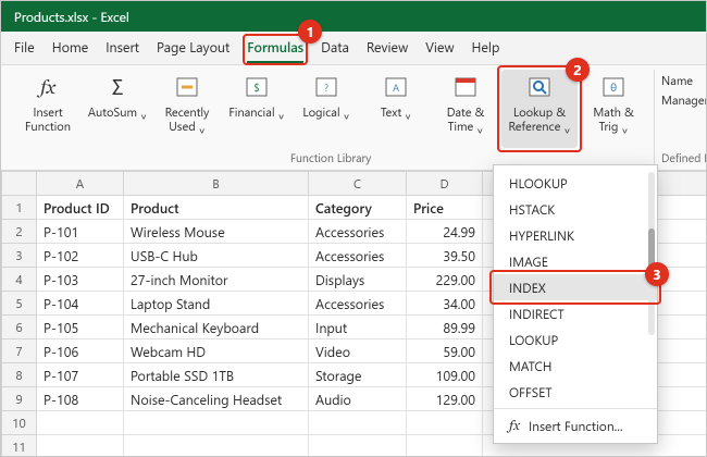
The function list is alphabetical, so MATCH, XLOOKUP and XMATCH are in the same menu. You can also select the fx button next to the formula bar and search for a function by name. If you have Microsoft 365 with Copilot, you can also describe the lookup in plain English; see how to use Copilot in Excel to create a formula, and check the formula it suggests before relying on it.

Exact match vs approximate match

The last argument of MATCH, match_type, is the most common source of wrong results. According to Microsoft’s MATCH function reference, the three options behave like this:

match_type	What MATCH finds	Data must be	Use it for
0	The first value exactly equal to the lookup value	In any order	IDs, names, codes, almost every lookup
1 or left out	The largest value less than or equal to the lookup value	Sorted smallest to largest	Price tiers, tax bands, grade cutoffs
-1	The smallest value greater than or equal to the lookup value	Sorted largest to smallest	Rare cases with descending thresholds

Why leaving out the 0 is risky: if your list isn’t sorted and you omit match_type, MATCH still returns a position without complaining, but it may be the wrong row or an #N/A for a value that is actually in the list. Nothing on screen tells you the answer is wrong. Typing the 0 every time avoids this.

When approximate match is the right tool: suppose J2:J5 holds order quantity thresholds 1, 10, 50 and 100, sorted ascending, and K2:K5 holds the discounts 0%, 5%, 10% and 15%. The formula =INDEX($K$2:$K$5,MATCH(75,$J$2:$J$5,1)) returns 10%, because 50 is the largest threshold that doesn’t exceed 75. An exact match would fail here, since 75 isn’t in the list.

Partial text matches: with match_type 0 you can use wildcards in text. An asterisk (*) stands for any number of characters and a question mark (?) stands for one character. =INDEX($D$2:$D$9,MATCH("Mech*",$B$2:$B$9,0)) returns 89.99, the price of the first product starting with “Mech”. To search for a real asterisk or question mark, put a tilde (~) in front of it.

Look up a value to the left

VLOOKUP can only return values from columns to the right of the column it searches. INDEX and MATCH don’t have that limit, because the search range and the return range are separate. To find the ID of a product by its name, search column B and return from column A:

=INDEX($A$2:$A$9,MATCH("Webcam HD",$B$2:$B$9,0))

The result is P-106, even though the ID column sits to the left of the name column. The same separation means that inserting or deleting columns elsewhere in the table doesn’t break the formula, because it never relies on a column number like VLOOKUP’s col_index_num.

The one rule to follow is that both ranges must start and end on the same rows. If MATCH searches A2:A9, INDEX should return from D2:D9, not D3:D10. A one-row offset doesn’t cause an error. It quietly returns the value from the next record.

Two-way lookup with INDEX, MATCH and MATCH

A two-way lookup finds the value where a row and a column meet, such as sales for one region in one quarter. You use INDEX with a two-dimensional range and two MATCH functions: one for the row number and one for the column number. This is sometimes called INDEX MATCH MATCH.

Suppose the quarterly sales table is in A12:E16, with quarter names in B12:E12 and regions in A13:A16:

Region	Q1	Q2	Q3	Q4
East	18,400	21,250	19,900	24,600
West	15,200	16,800	17,450	20,100
North	12,750	13,900	14,300	16,050
South	20,300	22,150	21,700	25,400

Type the region in H12 (West) and the quarter in H13 (Q3), then enter this formula in H14:

=INDEX($B$13:$E$16,MATCH(H12,$A$13:$A$16,0),MATCH(H13,$B$12:$E$12,0))

The first MATCH returns 2 (West is the second region) and the second returns 3 (Q3 is the third quarter), so INDEX returns 17,450 from row 2, column 3 of the data block. Notice that the INDEX range covers only the numbers, B13:E16, while the MATCH ranges cover the labels. The labels must line up with the edges of the INDEX range.

To make this easier to use, turn H12 and H13 into drop-down lists with Data Validation, so people pick from valid regions and quarters instead of typing them.

Look up with multiple criteria

Sometimes one column isn’t enough to identify a row. In a clothing price list, “Hoodie” might appear several times in different colors and sizes. Suppose A2:A7 holds the item, B2:B7 the color, C2:C7 the size and D2:D7 the price:

Item	Color	Size	Price
T-shirt	Blue	M	18.00
T-shirt	Blue	L	19.00
T-shirt	Black	M	18.50
Hoodie	Blue	L	42.00
Hoodie	Black	L	44.00
Hoodie	Black	M	43.00

With Hoodie in G2, Black in G3 and L in G4, this formula returns 44.00:

=INDEX($D$2:$D$7,MATCH(1,($A$2:$A$7=G2)*($B$2:$B$7=G3)*($C$2:$C$7=G4),0))

Here’s what happens. Each test in parentheses, such as $A$2:$A$7=G2, produces a list of TRUE and FALSE values, one per row. Multiplying the lists turns TRUE into 1 and FALSE into 0, so a row only gets a 1 when all three tests are true. MATCH then looks for the first 1, and INDEX returns the price from that row. You can add more conditions by multiplying more tests.

How to enter it: in Microsoft 365, Excel 2021, Excel 2024 and Excel for the web, just press Enter. In Excel 2019 and older on Windows, press Ctrl+Shift+Enter; Excel adds curly braces around the formula to show it’s a legacy array formula. Microsoft’s guide to dynamic array formulas explains the difference. If the formula returns #N/A in an older version even though the combination exists, it usually means it was entered with plain Enter.

A simpler option for shared files: add a helper column that joins the criteria, for example =A2&"|"&B2&"|"&C2 in E2, filled down. Then use an ordinary lookup: =INDEX($D$2:$D$7,MATCH(G2&"|"&G3&"|"&G4,$E$2:$E$7,0)). This needs no special keystroke in any version and is easier for others to read. The separator character stops combinations like “AB” + “C” and “A” + “BC” from looking identical.

More useful INDEX and MATCH patterns

Look up across a row instead of a column

MATCH works on horizontal ranges too, so INDEX and MATCH can replace HLOOKUP. Using the sales table, =INDEX($B$13:$E$13,MATCH("Q4",$B$12:$E$12,0)) returns East’s Q4 figure, 24,600.

Return a whole column or row

If you set row_num or column_num to 0, INDEX returns the entire column or row of the range, as Microsoft’s INDEX function reference describes. Combined with MATCH, this lets a formula pick which column to total: =SUM(INDEX($B$13:$E$16,0,MATCH("Q2",$B$12:$E$12,0))) adds up the Q2 column and returns 74,100. In Microsoft 365, entering the INDEX part on its own spills all four values into the cells below; if those cells aren’t empty you will see a #SPILL! error.

Find the item with the highest or lowest value

Use MAX or MIN as the lookup value. =INDEX($B$2:$B$9,MATCH(MAX($D$2:$D$9),$D$2:$D$9,0)) returns 27-inch Monitor, the most expensive product. If two items tie, MATCH returns the first one.

Check whether a value exists

=ISNUMBER(MATCH(G2,$A$2:$A$9,0)) returns TRUE if the ID in G2 is in the list and FALSE if it isn’t, without showing an error. This is handy for validating entries or for conditional formatting rules.

Look up from another sheet or an Excel table

Ranges can point to another worksheet: =INDEX(Prices!$D$2:$D$500,MATCH(A2,Prices!$A$2:$A$500,0)). If the sheet name contains spaces, wrap it in single quotes, such as 'Price List'!$D$2:$D$500. If your data is formatted as an Excel table (Home > Format as Table), you can use column names instead of cell ranges, for example =INDEX(Products[Price],MATCH(G2,Products[Product ID],0)). Table references grow automatically as you add rows, so you don’t need to update the ranges.

Case-sensitive lookup

MATCH treats uppercase and lowercase as the same. To tell “ab-100” from “AB-100”, combine it with EXACT: =INDEX($D$2:$D$9,MATCH(TRUE,EXACT(G2,$A$2:$A$9),0)). This is an array formula, so use Ctrl+Shift+Enter in Excel 2019 and older.

Fix INDEX and MATCH errors

#N/A: the value wasn’t found

• Extra spaces. “P-105 ” with a trailing space won’t match “P-105”. Clean the data with TRIM, or wrap the lookup value: MATCH(TRIM(G2),...).
• Numbers stored as text. An ID typed as the number 1001 won’t match the text “1001”. Look for a small green triangle in the cell corner, or make both sides the same type.
• Missing 0. If match_type is left out on unsorted data, results are unreliable. Add the 0.
• The value really isn’t there. Use IFNA, as in Step 6, to show a clear message.
• A multiple-criteria formula in an older version may need Ctrl+Shift+Enter.

Wrong value returned

• The INDEX range and MATCH range start on different rows, so every answer comes from a neighboring record. Make them start and end on the same rows.
• match_type is 1 or missing on unsorted data. Change it to 0.
• The ranges weren’t locked with dollar signs and shifted when the formula was copied.

#REF!

INDEX was asked for a position outside its range, for example row 12 of a 10-row range. This happens when the MATCH range is longer than the INDEX range. Make both ranges the same size.

#NAME?

A function name is misspelled, text in the formula is missing its quotation marks, or you are using XMATCH or XLOOKUP in a version that doesn’t have them.

The formula shows as text

If the cell displays the formula itself instead of a result, the cell may be formatted as Text or Show Formulas may be turned on. See why Excel shows formulas instead of results for the fixes.

How to undo or remove the formula

Press Ctrl+Z (Command+Z on a Mac) right after a change to undo it. To keep the results but remove the formulas, select the cells, copy them, then use Home > Paste > Paste Values. Do this only when you no longer need the results to update, because pasted values won’t change if the source data does.

INDEX and MATCH vs XLOOKUP vs VLOOKUP

Microsoft now recommends XLOOKUP and XMATCH as improved versions of the older lookup functions in its overview of looking up values with VLOOKUP, INDEX or MATCH. Each approach still has its place:

Feature	INDEX and MATCH	XLOOKUP	VLOOKUP
Available in	All current versions	Microsoft 365, Excel 2021, Excel 2024, web	All current versions
Default match	Approximate (type 0 for exact)	Exact	Approximate (type FALSE for exact)
Look left	Yes	Yes	No
Survives inserted columns	Yes	Yes	No, the column number can point to the wrong column
Two-way lookup	Yes, with two MATCH functions	Yes, by nesting XLOOKUP	Only with MATCH added
Built-in “not found” text	No, wrap in IFNA	Yes, if_not_found argument	No, wrap in IFNA
Search last to first	Not directly	Yes	No

Choose XLOOKUP if everyone who opens the file has Microsoft 365, Excel 2021 or later. It’s shorter to write and exact by default; see how to use XLOOKUP in Excel. Choose INDEX and MATCH when the workbook must work in Excel 2019 or 2016, when you want a two-way lookup in one readable formula, or when you are editing existing workbooks that already use it. VLOOKUP is fine for quick, simple lookups where the search column is on the left; see how to use VLOOKUP in Excel for that method.

If you have Microsoft 365 or Excel 2021 or later, you can also swap MATCH for XMATCH inside INDEX. XMATCH is exact by default and can search from the last item to the first, for example =INDEX($D$2:$D$9,XMATCH(G2,$A$2:$A$9,0,-1)) to find the last occurrence of a value.

INDEX and MATCH also work the same way in Google Sheets. If you use both programs, how to use VLOOKUP in Google Sheets covers the Sheets lookup functions.

Frequently Asked Questions

What is the basic INDEX and MATCH formula?

The basic formula is =INDEX(return_range, MATCH(lookup_value, lookup_range, 0)). The return range is the column holding the answer, the lookup range is the column you search, and the 0 forces an exact match. Both ranges should cover the same rows.

Why use INDEX and MATCH instead of VLOOKUP?

INDEX and MATCH can return values from columns to the left of the search column, aren’t broken by inserting or deleting columns, and can do two-way lookups. VLOOKUP needs the search column on the far left and uses a fixed column number that can point to the wrong column after the table changes.

Is XLOOKUP better than INDEX and MATCH?

For most new workbooks in Microsoft 365, Excel 2021 or Excel 2024, XLOOKUP is easier because it is one function and exact by default. INDEX and MATCH remain the better choice when files must work in Excel 2019 or older, since those versions can’t calculate XLOOKUP.

What does the 0 at the end of MATCH mean?

It sets match_type to exact match, so MATCH only returns a position when it finds a value exactly equal to the one you are searching for. Without it, MATCH uses approximate matching, which expects the list to be sorted in ascending order and can return the wrong row on unsorted data.

Can INDEX and MATCH return more than one result?

MATCH always returns the first match it finds, so the standard formula returns one value. To list every matching row in Microsoft 365, Excel 2021 or Excel 2024, the FILTER function is a better fit. In older versions, a helper column that numbers each match is the usual workaround.

Do I need to press Ctrl+Shift+Enter for INDEX and MATCH?

Not for the standard single-criterion formula, which works with Enter in every version. Only array formulas, such as the multiple-criteria and case-sensitive versions, need Ctrl+Shift+Enter, and only in Excel 2019 and older. Microsoft 365, Excel 2021, Excel 2024 and Excel for the web calculate them with Enter.

Does INDEX and MATCH work on a Mac and in Excel for the web?

Yes. The functions and syntax are the same in Excel for Mac and Excel for the web. The main difference on a Mac is the shortcut for adding dollar signs, which is Command+T instead of F4.

Why does my INDEX and MATCH return the wrong row?

The two most common causes are a missing 0 in MATCH and ranges that start on different rows. Check that match_type is 0 and that the INDEX range and MATCH range begin and end on the same rows, for example D2:D9 and A2:A9.

Next steps

Start with the simple pattern from the steps above, test the MATCH part on its own whenever a result looks wrong, and always include the 0. Once that feels comfortable, try the two-way lookup on your own report tables. If everyone using the file has a recent version of Excel, compare the same lookup written with XLOOKUP and keep whichever one is easier for you and your colleagues to read.