Finding the average (mean) of a set of numbers in Google Sheets takes one formula: AVERAGE. Sheets also shows a quick average when you select cells, and it has variations for averaging only the cells that meet a condition, skipping zeros, or including text values. This guide covers all of them with examples you can copy.
Quick Answer
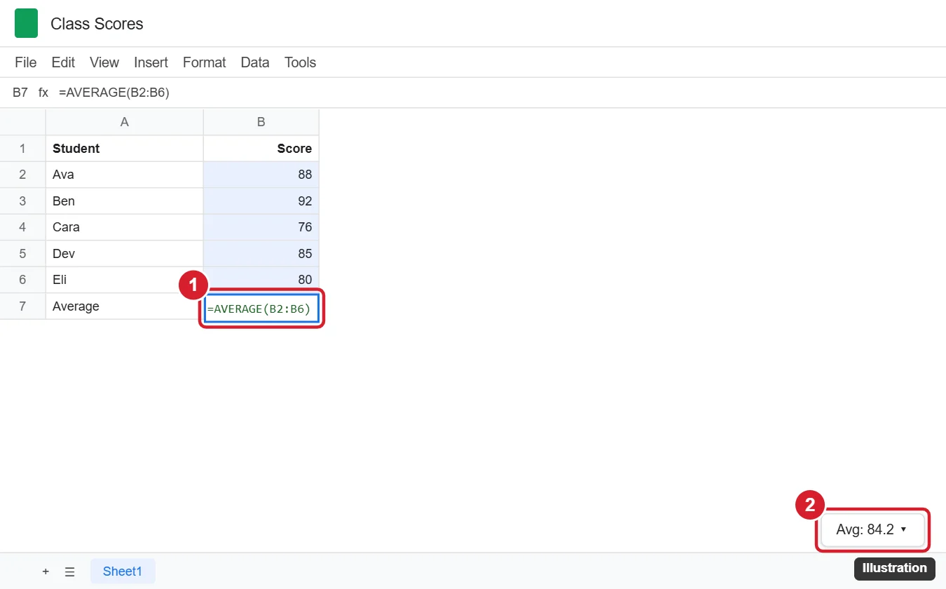
Click an empty cell, type =AVERAGE(B2:B6) (replace the range with your cells), and press Enter. For a quick look without a formula, select the cells and check the Avg value in the bottom-right corner.
Method 1: The AVERAGE Function
- Click the cell where you want the result.
- Type
=AVERAGE(. - Drag over the cells to average, or type the range, such as
B2:B6. - Type
)and press Enter.
You can average separate ranges or individual cells too: =AVERAGE(B2:B6, D2:D6) or =AVERAGE(B2, B4, B6). AVERAGE ignores empty cells and text but includes zeros.
Method 2: Use the Functions Menu
- Select the cells you want to average (or the empty cell below them).
- Click the Functions button (Σ) on the toolbar.
- Choose AVERAGE. Sheets inserts the formula; adjust the range and press Enter.
Method 3: Quick Average Without a Formula
Select a range of numbers. The summary box in the bottom-right corner shows Sum by default; click it and choose Avg to see the average. This doesn’t add anything to the sheet.
Average with Conditions: AVERAGEIF and AVERAGEIFS
- One condition:
=AVERAGEIF(A2:A20, "East", C2:C20)averages sales in column C where the region in column A is “East.” - Numbers above a value:
=AVERAGEIF(C2:C20, ">50") - Multiple conditions:
=AVERAGEIFS(C2:C20, A2:A20, "East", B2:B20, ">=2026-01-01")averages East sales from 2026 onward.
Average Without Zeros
Use =AVERAGEIF(B2:B20, "<>0") to skip cells containing 0. This is useful when zeros mean “no data” rather than an actual score.
Other Averaging Functions
| Function | What it does |
|---|---|
AVERAGEA |
Counts text as 0 and TRUE as 1, FALSE as 0 |
AVERAGE.WEIGHTED |
Weighted average: =AVERAGE.WEIGHTED(B2:B6, C2:C6) with weights in C |
MEDIAN |
Middle value, less affected by outliers |
MODE |
Most frequent value |
TRIMMEAN |
Average after excluding a percentage of highest and lowest values |
Round the Result
Wrap the formula in ROUND to control decimals: =ROUND(AVERAGE(B2:B6), 1). Or keep the full value and use Format > Number or the decrease-decimal button to change how many decimals display.
Troubleshooting
- #DIV/0! error: the range has no numbers. Check the range or use
=IFERROR(AVERAGE(B2:B6), ""). - Numbers ignored: they may be stored as text (left-aligned). Select them and choose Format > Number > Number, or use Data > Data cleanup tools.
- Average seems too low: zeros are included. Use AVERAGEIF with “<>0” if that’s not what you want.
- Result changes when adding rows: use an open-ended range like
B2:Bto include new rows automatically (make sure the formula isn’t inside that range).
Related: Calculate correlation in Google Sheets.
Frequently Asked Questions
Does AVERAGE include blank cells?
No. Blank cells are skipped, but cells containing 0 are included.
How do I average an entire column?
Use =AVERAGE(B:B) in a cell outside column B, or =AVERAGE(B2:B) to skip a header.
Can I average across sheets?
Yes: =AVERAGE(Sheet1!B2:B10, Sheet2!B2:B10).
Summary
- Type
=AVERAGE(range)and press Enter. - Select cells and read Avg in the bottom-right for a quick check.
- Use
AVERAGEIForAVERAGEIFSfor conditions. - Use
"<>0"to skip zeros and ROUND to tidy decimals.

Kermit Matthews runs Live2Tech from just outside Philadelphia. He is an IT specialist with over 20 years of experience, from a university help desk to small-business IT, IT management and his own consulting practice, and has written tech guides full time since 2020. Steps are checked against the current software on a real device or the maker’s official documentation. More about Kermit.