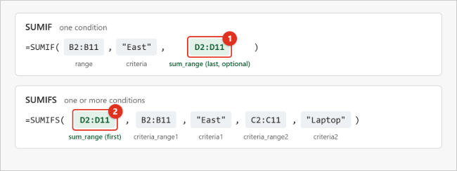
To add up only the numbers that match a condition in Excel, use SUMIF for one condition and SUMIFS for two or more. Click an empty cell and type =SUMIF(B2:B11,"East",D2:D11) to total column D wherever column B says East, or =SUMIFS(D2:D11,B2:B11,"East",C2:C11,"Laptop") to total only the East rows that are also laptops. The one thing to remember: SUMIF puts the column to add last, and SUMIFS puts it first.
This guide walks through both functions with a small sample sheet you can copy, then covers every kind of criteria (text, numbers, dates, wildcards, blanks and cell references), OR conditions, and the fixes for the most common errors and wrong totals.
What you need and which versions this covers
SUMIF and SUMIFS work the same way in Excel for Microsoft 365 on Windows and Mac, Excel 2024, Excel 2021, Excel 2019, Excel 2016 and Excel for the web, according to Microsoft’s function reference pages. You don’t need any add-ins. You only need:
- A range of cells to check (for example, a Region column).
- A range of numbers to add that lines up row by row with the range you check (for example, an Amount column).
- The condition you want to match, typed into the formula or stored in a cell.
A few terms used throughout: a range is a block of cells such as B2:B11. A criterion (plural criteria) is the rule a cell must meet, such as "East" or ">1000". The sum range is the set of cells that actually gets added.
SUMIF vs. SUMIFS at a glance
Both functions add numbers from rows that pass a test. The difference is how many tests they allow and the order of their arguments (the values you put inside the parentheses).
| SUMIF | SUMIFS | |
|---|---|---|
| Syntax | =SUMIF(range, criteria, [sum_range]) |
=SUMIFS(sum_range, criteria_range1, criteria1, [criteria_range2, criteria2], ...) |
| Number of conditions | One | One or more, up to 127 range and criteria pairs |
| Where the cells to add go | Last, and optional | First, and required |
| How conditions combine | Not applicable | AND: a row is added only if it meets every condition |
| Range sizes | Should match; if they don’t, Excel resizes the sum range to match the range | Must match, or the formula returns #VALUE! |
Square brackets in a syntax line mean the argument is optional. In SUMIF, if you leave out sum_range, Excel adds the same cells it checked. That’s handy when the condition is about the numbers themselves, such as “amounts over 1,000.”
Which should you use? If you only ever have one condition, either works. Many people use SUMIFS even for a single condition so every formula in the workbook has the same argument order, which makes them easier to read and harder to mix up. Microsoft’s own SUMIFS page calls the different argument order a common source of problems when people copy and edit these formulas.
The sample data used in this guide
Type or paste this small sales list into a blank worksheet, starting in cell A1, to follow along. The headings are in row 1 and the data is in rows 2 to 11.
| Row | A: Date | B: Region | C: Product | D: Amount |
|---|---|---|---|---|
| 2 | 1/6/2026 | East | Laptop | 1,200 |
| 3 | 1/9/2026 | West | Monitor | 300 |
| 4 | 1/14/2026 | East | Monitor | 250 |
| 5 | 1/20/2026 | North | Laptop | 1,350 |
| 6 | 1/27/2026 | West | Keyboard | 80 |
| 7 | 2/3/2026 | East | Keyboard | 95 |
| 8 | 2/10/2026 | North | Monitor | 320 |
| 9 | 2/17/2026 | West | Laptop | 1,100 |
| 10 | 2/24/2026 | East | Laptop | 1,250 |
| 11 | 3/2/2026 | North | Keyboard | 70 |
The grand total of column D is 6,015. Every result below was calculated from this data, so you can check your own formulas against it. If you just need the plain total of a column, see how to sum a column in Excel.
How to use SUMIF (one condition)
Goal: total all sales in the East region.
Step 1: Select the cell for the result
Click an empty cell outside the data, such as F2. Putting the formula outside the ranges it reads avoids accidentally including the result in its own total.
Step 2: Start the formula and select the range to check
Type =SUMIF( and then select B2:B11, the Region column, with your mouse, or type B2:B11. Excel shows a small tooltip under the cell with the argument names, and the one you’re on appears in bold. Type a comma.
Step 3: Enter the criteria
Type "East" with the double quotation marks, then another comma. Text criteria and anything that includes a comparison symbol must be inside double quotes. A plain number such as 300 doesn’t need them.
Step 4: Select the cells to add and finish
Select D2:D11, the Amount column, type a closing parenthesis, and press Enter. The complete formula is:
=SUMIF(B2:B11,"East",D2:D11)
The cell shows 2,795, which is 1,200 + 250 + 95 + 1,250, the four East rows.
Step 5: Check the result
Click the cell and look at the formula bar to confirm the ranges. To double-check the total, filter column B to East and select the visible amounts; the Sum on the status bar at the bottom of the window should match. Matching text isn’t case-sensitive, so “east” and “EAST” find the same rows.

How to use SUMIFS (several conditions)
Goal: total laptop sales in the East region only.
Step 1: Select an empty cell
Click a blank cell such as F3.
Step 2: Enter the range to add first
Type =SUMIFS(, select D2:D11, and type a comma. This is the step people most often get wrong when they switch from SUMIF, because the amounts now come first.
Step 3: Add the first range and its condition
Select B2:B11, type a comma, then type "East" and another comma. Each condition is always a pair: the range to check followed by what to look for in it.
Step 4: Add the second range and its condition
Select C2:C11, type a comma, type "Laptop", add a closing parenthesis and press Enter:
=SUMIFS(D2:D11,B2:B11,"East",C2:C11,"Laptop")
The result is 2,450 (rows 2 and 10). Rows that match only one condition, such as the East monitor in row 4 or the North laptop in row 5, are left out.
Step 5: Add more conditions if you need them
Keep adding range and criteria pairs. For example, =SUMIFS(D2:D11,B2:B11,"East",C2:C11,"Laptop",A2:A11,">="&DATE(2026,2,1)) adds a date condition and returns 1,250, the only East laptop sold on or after February 1. Every range you add must be the same size as the sum range, here 10 rows tall.
Build the formula with the Function Arguments box
If you’d rather fill in labeled boxes than remember the argument order, use Excel’s built-in function helper. This is the easiest way to avoid putting the ranges in the wrong order.
Step 1: Open Insert Function
Click the result cell, then select Insert Function (the fx button to the left of the formula bar). You can also go to the Formulas tab and look in the Math & Trig list of the Function Library group.
Step 2: Find SUMIFS
In the Insert Function box, type sumifs in the search box and select Go, or pick a category from the drop-down. Double-click SUMIFS in the Select a function list.
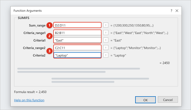
Step 3: Fill in the boxes
The Function Arguments box opens with one field per argument. Click in Sum_range and select D2:D11, click in Criteria_range1 and select B2:B11, then type East in Criteria1. If you type text without quotes, Excel normally adds them when you move to the next box. As you fill in each pair, a new Criteria_range2 and Criteria2 pair appears. The live result appears near the bottom of the box next to Formula result.
Step 4: Select OK
Select OK to place the finished formula in the cell. If something looks off, Help on this function opens Microsoft’s reference page for SUMIFS. On a Mac, the same button may open a side pane rather than a separate box, but the argument names are the same.
How to write criteria: text, numbers, wildcards and cell references
Criteria work the same way in SUMIF and SUMIFS. The table shows the patterns you’ll use most, with results from the sample data.
| To add amounts where… | Formula | Result |
|---|---|---|
| Region equals East | =SUMIF(B2:B11,"East",D2:D11) |
2,795 |
| Region is anything except East | =SUMIF(B2:B11,"<>East",D2:D11) |
3,220 |
| Amount is greater than 1,000 | =SUMIF(D2:D11,">1000") |
4,900 |
| Amount is between 100 and 1,000 | =SUMIFS(D2:D11,D2:D11,">=100",D2:D11,"<=1000") |
870 |
| Product starts with “Key” | =SUMIF(C2:C11,"Key*",D2:D11) |
245 |
| Region has exactly four letters | =SUMIF(B2:B11,"????",D2:D11) |
4,275 |
| Region matches the text in cell G1 | =SUMIF(B2:B11,G1,D2:D11) |
Depends on G1 |
| Amount is greater than the number in G2 | =SUMIF(D2:D11,">"&G2) |
Depends on G2 |
The rules behind those patterns:
- Comparison operators are
=(equal to),>(greater than),<(less than),>=(greater than or equal to),<=(less than or equal to) and<>(not equal to). Put the operator and the value together inside one set of quotes, as in">1000". - Wildcards match partial text. An asterisk (
*) stands for any number of characters, so"*top*"matches any product containing “top.” A question mark (?) stands for exactly one character. To look for a real asterisk or question mark, put a tilde in front of it:"~*"or"~?". Wildcards apply to text, not to numbers. - Cell references make a formula reusable. Type the condition in a cell such as G1 and point the criteria at that cell with no quotes. Change G1, and the total updates.
- Operator plus a cell needs the ampersand (
&), which joins text together.">"&G2means “greater than whatever is in G2.” Writing">G2"instead would look for amounts greater than the text “G2” and return 0. - Partial match on a cell value combines both ideas:
"*"&G1&"*"adds rows whose text contains whatever is in G1. - Blank and non-blank cells:
""matches empty cells and"<>"matches cells that aren’t empty. For example,=SUMIFS(D2:D11,C2:C11,"<>")adds only rows that have a product name. - Functions can be criteria too, such as
">"&AVERAGE(D2:D11)to add sales above the average.
The same criteria rules apply to the counting functions. For counting matching cells instead of adding numbers, see how to count a word in Excel with COUNTIF.
Sum by date and date range
Excel stores dates as serial numbers and only displays them as dates, so date criteria work just like number criteria. The safest way to write a date inside a formula is the DATE(year, month, day) function, because it gives the same result no matter whether the computer uses month-first or day-first date settings. A typed date in quotes, like ">=2/1/2026", works on a US-format system but can be read differently elsewhere.
One date or everything after a date
=SUMIF(A2:A11,">="&DATE(2026,2,1),D2:D11) adds every sale on or after February 1, 2026, and returns 2,835. To match a single day, drop the operator: =SUMIF(A2:A11,DATE(2026,1,20),D2:D11) returns 1,350.
A date range (between two dates)
A range needs two conditions on the same date column, so use SUMIFS:
=SUMIFS(D2:D11,A2:A11,">="&DATE(2026,1,1),A2:A11,"<"&DATE(2026,2,1))
This totals January 2026 and returns 3,180. Using “less than the first day of next month” instead of “less than or equal to January 31” also catches entries that include a time of day, such as 1/31/2026 3:00 PM.
Start and end dates in cells
Put a start date in G1 and an end date in G2, then use =SUMIFS(D2:D11,A2:A11,">="&G1,A2:A11,"<="&G2). Anyone can change the two dates without touching the formula. For a rolling window, replace the cells with TODAY(), for example ">="&TODAY()-30 for the last 30 days. TODAY() recalculates whenever the workbook recalculates, so the result changes from day to day. If you need help entering or formatting dates, see how to insert a date and time in Excel.
Sum with OR conditions
SUMIFS only does AND: every condition must be true. When you want rows that meet one condition or another, use one of these approaches.
Add two SUMIF results
=SUMIF(C2:C11,"Laptop",D2:D11)+SUMIF(C2:C11,"Monitor",D2:D11) returns 5,770, the total of all laptops and monitors. This is easy to read and works in every version.
Use an array constant inside SUM
=SUM(SUMIF(C2:C11,{"Laptop","Monitor"},D2:D11)) gives the same 5,770 in one function. The curly braces hold a list of values, SUMIF returns one total for each, and SUM adds them. You can do the same with SUMIFS, for example =SUM(SUMIFS(D2:D11,C2:C11,"Laptop",B2:B11,{"East","West"})) to total laptops sold in either East or West, which returns 3,550.
Avoid double counting when both conditions are in different columns
If the OR conditions check different columns, such as “region is East or amount is over 1,000,” a row can meet both and would be added twice. Subtract the overlap with a SUMIFS that requires both: =SUMIF(B2:B11,"East",D2:D11)+SUMIF(D2:D11,">1000")-SUMIFS(D2:D11,B2:B11,"East",D2:D11,">1000"). The result is 2,795 + 4,900 − 2,450 = 5,245. For many OR conditions, SUMPRODUCT or FILTER (described in the FAQ) can be clearer.
More worked examples
A region summary that updates itself
Type East, West and North in F2:F4. In G2, enter =SUMIF($B$2:$B$11,F2,$D$2:$D$11) and drag the fill handle down to G4. The dollar signs make the data ranges absolute references, so they stay fixed while the criteria cell moves from F2 to F3 to F4. The results are East 2,795, West 1,480 and North 1,740, which add up to the grand total of 6,015. That last check is worth doing on any summary: if the parts don’t add up to the whole, some rows have a spelling or spacing difference.
A product-by-region grid with SUMIFS
Put regions down F2:F4 and products across G1:I1 (Laptop, Monitor, Keyboard). In G2, enter =SUMIFS($D$2:$D$11,$B$2:$B$11,$F2,$C$2:$C$11,G$1) and fill it across and down. The mixed references ($F2 and G$1) lock the column of the region labels and the row of the product labels. East laptops show 2,450, North monitors 320, and so on.

Use an Excel table so new rows are included
Click inside the data and press Ctrl + T (or select Insert > Table) to turn it into an Excel table, then name it Sales on the Table Design tab. You can now write =SUMIFS(Sales[Amount],Sales[Region],"East"). These structured references grow automatically when you add rows to the table, so you never have to edit the ranges.
Totals for every category in one formula
In Excel for Microsoft 365, Excel 2024, Excel 2021 and Excel for the web, the UNIQUE function can feed SUMIF a list of criteria: =SUMIF(B2:B11,UNIQUE(B2:B11),D2:D11). Pair it with =UNIQUE(B2:B11) in the column to its left, and both results spill down the sheet. Older versions don’t have UNIQUE, so type the list yourself and copy SUMIF down as in the first example.
Percentage of the total
Divide a conditional total by the grand total: =SUMIF(B2:B11,"East",D2:D11)/SUM(D2:D11) returns about 0.465. Select Percent Style (%) in the Number group on the Home tab to show 46%. Don’t also multiply by 100, or you’ll see 4,647%.
Why SUMIF or SUMIFS returns 0, #VALUE! or the wrong total
The result is 0
- Missing quotes. Text and operator criteria must be quoted.
=SUMIF(D2:D11,>1000)won’t even be accepted, and">G2"compares against the letters G2. Use">1000"or">"&G2. - Extra spaces or typos. “East ” with a trailing space doesn’t match “East.” Imported data often carries hidden spaces. Clean a copy of the column with
=TRIM(B2), or use a wildcard such as"East*"as a quick test. - Numbers stored as text. Values pasted from other systems can be text that only looks like numbers. They’re often aligned to the left and may show a small green triangle. SUMIF skips them. Select the cells, click the warning icon and choose Convert to Number.
- Dates stored as text. If a date criterion matches nothing, check that column A holds real dates. A real date changes its look when you apply a different date format; text doesn’t.
- Arguments in the wrong order. A SUMIF converted to SUMIFS without moving the sum range will check the amounts against “East” and find nothing.
The result is #VALUE!
- SUMIFS ranges are different sizes. Microsoft says every criteria range in SUMIFS must have the same number of rows and columns as the sum range.
=SUMIFS(D2:D11,B2:B9,"East")fails because B2:B9 is shorter. Make them match. - The formula points to a closed workbook. SUMIF and SUMIFS that refer to cells in another workbook return #VALUE! when that file is closed. Open the other workbook and press F9 to recalculate.
- A criteria string is longer than 255 characters. Microsoft notes these functions return incorrect results when matching strings longer than 255 characters. Shorten the text, or split it into pieces joined with
&.
The total is wrong but there’s no error
- The ranges don’t start on the same row. SUMIF doesn’t complain about
=SUMIF(B2:B11,"East",D3:D12); it quietly shifts the sum one row down and adds the wrong cells. Always start both ranges on the same row. SUMIF also resizes a mismatched sum range to match the size of the range, starting from its first cell, which can hide mistakes. - The sum range has TRUE or FALSE values. In SUMIFS, cells containing TRUE count as 1 and FALSE as 0, which can change the total.
- The formula is inside its own range. A formula like
=SUMIF(D:D,">1000")placed in column D creates a circular reference. Put it in a different column. - Calculation is set to manual. If totals don’t change when data changes, go to Formulas > Calculation Options and choose Automatic, or press F9.
- The formula shows as text. If the cell displays the formula instead of a number, the cell may be formatted as Text. See why Excel shows formulas instead of results.
To undo a formula you no longer want, select the cell and press Delete, or press Ctrl + Z (Command + Z on a Mac) right after entering it. SUMIF and SUMIFS never change the source data, so removing them is safe.
Frequently Asked Questions
What is the difference between SUMIF and SUMIFS?
SUMIF adds numbers that meet one condition, with the syntax =SUMIF(range, criteria, [sum_range]). SUMIFS adds numbers that meet every one of several conditions, with the syntax =SUMIFS(sum_range, criteria_range1, criteria1, ...). The cells to add come last in SUMIF and first in SUMIFS.
Can SUMIF use more than one condition?
Not by itself. For conditions that must all be true, use SUMIFS. For either-or conditions on the same column, add two SUMIF formulas together or use =SUM(SUMIF(range,{"A","B"},sum_range)).
Can I use SUMIFS with just one condition?
Yes. =SUMIFS(D2:D11,B2:B11,"East") returns the same 2,795 as the SUMIF version. Some people prefer it so all their conditional sums use the same argument order.
Is SUMIF case-sensitive?
No. “east,” “East” and “EAST” all match. If you need an exact-case match, use =SUMPRODUCT(--EXACT(B2:B11,"East"),D2:D11). EXACT compares text with case, and the two minus signs turn its TRUE and FALSE results into 1 and 0.
How many conditions can SUMIFS handle?
Up to 127 range and criteria pairs, according to Microsoft. In practice, a formula with more than four or five conditions is easier to manage with cell references or a PivotTable.
Can SUMIF add numbers from another sheet?
Yes. Include the sheet name in the ranges, such as =SUMIF(Sales!B2:B11,"East",Sales!D2:D11). If the ranges are in another workbook, keep that workbook open or the formula returns #VALUE!.
What can I use instead of SUMIFS for complex conditions?
SUMPRODUCT handles OR logic and calculations in one formula, for example =SUMPRODUCT(((B2:B11="East")+(B2:B11="West"))*D2:D11), which returns 4,275. In versions with dynamic arrays, =SUM(FILTER(D2:D11,(B2:B11="East")*(C2:C11="Laptop"))) also returns 2,450 and lets you display the matching rows if you drop the SUM. A PivotTable is the better choice when you want many totals at once.
Do SUMIF and SUMIFS work in Google Sheets?
Yes. Google Sheets uses the same argument order, with the range to sum first in SUMIFS, so the basic SUMIF and SUMIFS formulas in this guide carry over. Array tricks such as the curly-brace lists may need ARRAYFORMULA in Sheets.
Does SUMIF ignore blank cells and text?
Yes. Blank cells and text in the sum range aren’t added and don’t cause an error. That’s also why numbers stored as text are silently skipped.
Next steps
Start with one SUMIF on your own data, check it against a filter and the status bar, and then switch to SUMIFS when you need a second condition. Once the argument order feels natural, move the conditions into cells so one formula can answer many questions. For the full list of arguments and Microsoft’s own examples, see the SUMIF function and SUMIFS function reference pages, and Microsoft’s guide to fixing #VALUE! errors in SUMIF and SUMIFS.

Kermit Matthews runs Live2Tech from just outside Philadelphia. He is an IT specialist with over 20 years of experience, from a university help desk to small-business IT, IT management and his own consulting practice, and has written tech guides full time since 2020. Steps are checked against the current software on a real device or the maker’s official documentation. More about Kermit.