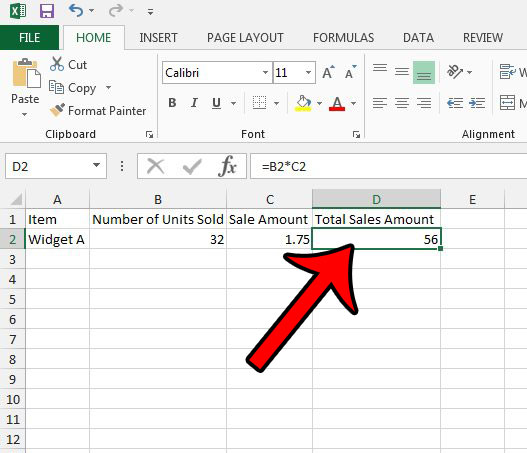
A cell in a Microsoft Excel spreadsheet can contain many different types of information. Some of those types of information, such as numerical values, can even represent different types of data. For example, you might have a spreadsheet that contains sales information, where one column indicates the number of units that were sold, and another column indicates the monetary value of those sales.
When there are a lot of similar types of data in nearby columns, it can be difficult to differentiate monetary values from numerical values. Fortunately Excel 2013 offers a number of different formatting choices, so you can apply one of those formatting types to your dollar values and display the $ symbol to the left of them.
Displaying the $ Symbol Next to a Number in Excel 2013
The steps in this article are going to show you how to format a cell with the Currency format. The end result will be a cell that displays a number with dollar sign and two decimal places. If you have UPC numbers in one of your spreadsheets, then you might be having a lot of trouble with their formatting, too. Click here to see how you can format difficult numbers like that.
Step 1: Open your spreadsheet in Excel 2013.
Step 2: Select the cell in which you would like to display the dollar symbol to the left of the number.

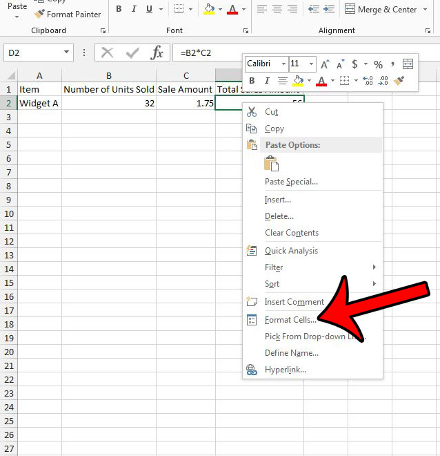
Step 3: Right-click the cell, then click the Format Cells option.

Step 4: Click the Currency option under Category at the left side of the window. Confirm that there is a $ symbol in the Symbol field, and a 2 to the right of Decimal places. You can then click the OK button at the bottom of the window.

If you have a spreadsheet that displays an unwanted percentage symbol, then this article can show you how to remove it.

Kermit Matthews is a freelance writer based in Philadelphia, Pennsylvania with more than a decade of experience writing technology guides. He has a Bachelor’s and Master’s degree in Computer Science and has spent much of his professional career in IT management.
He specializes in writing content about iPhones, Android devices, Microsoft Office, and many other popular applications and devices.