Sometimes when you are creating a spreadsheet you will focus first on adding all of the data, then format everything so that it is more presentable for your audience. This could include things like making it look better when you print, or applying the correct type of formatting for your data.
But you may discover that you have added data that your audience doesn’t need to see, or may create some confusion. While your initial thought could be to simply delete the column with that data, it’s possible that you could need that data later, or that it is part of a formula. One way to resolve this is to hide that column. This keeps the data in the spreadsheet, but removes it from view.
Hiding Columns in Google Sheets
The steps in this article were performed in the desktop version of the Google Chrome Web browser, but will also work in other desktop browsers like Firefox or Edge.
Step 1: Sign into your Google Drive at https://drive.google.com and open the Sheets file containing the column you want to hide.
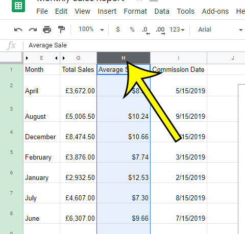
Step 2: Click the column letter that you want to hide at the top of the spreadsheet.

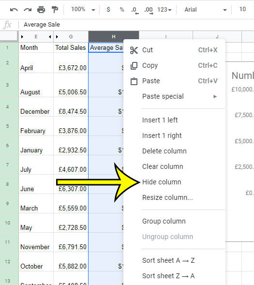
Step 3: Right-click the selected column letter, then choose the Hide column option.

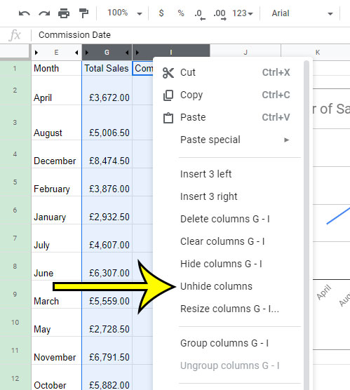
If you decide later to unhide the column, select the column to the left and to the right of the hidden column, then choose the Unhide column option.

You can hide other things in Google Sheets, too, such as an entire worksheet. Find out how to hide a worksheet tab in Google Sheets if there’s an entire sheet that you don’t want to be visible.

Kermit Matthews is a freelance writer based in Philadelphia, Pennsylvania with more than a decade of experience writing technology guides. He has a Bachelor’s and Master’s degree in Computer Science and has spent much of his professional career in IT management.
He specializes in writing content about iPhones, Android devices, Microsoft Office, and many other popular applications and devices.