When you first start working with Microsoft Excel and are familiarizing yourself with some basic formulas, you may not give much thought to the names of the other worksheets in your Excel workbook. But as you start to take advantage of all of the complex formulas and the usefulness that additional worksheets offer, you may discover that the default naming structure of Excel tabs isn’t that useful.
Excel worksheets can have a lot of tabs. You may be used to seeing some spreadsheets with a handful of sheets, especially since some Excel versions include 3 sheets by default, but it is common for some users to have dozens of sheets.
When you are working with a large, multi-worksheet Excel workbook, properly naming your worksheet tabs becomes incredibly important. The default naming structure of Sheet1, Sheet2, etc. becomes unhelpful and finding the correct data can be cumbersome. Fortunately, you are able to rename worksheet tabs in Excel 2016 and make it much easier to find the sheet that you need.
How to Rename Sheet in Excel 2010, 2013, or 2016
- Open your Excel file.
- Find the worksheet tab at the bottom of the window.
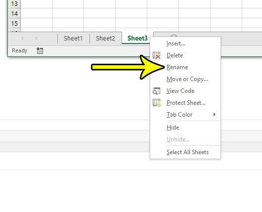
- Right-click on the tab and choose Rename.
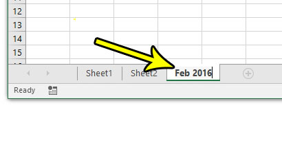
- Type the new name, then press Enter.
Our article continues below with additional information on changing a tab name in Excel 2016, including pictures of these steps.
How to Change the Name of a Worksheet Tab in Excel 2016 (Guide with Pictures)
The steps in this article will show you how to change the name of a worksheet tab. If you have any formulas in your spreadsheet that reference a cell on that worksheet, those formulas will update automatically with the new tab name.
Step 1: Open your spreadsheet in Excel 2016.
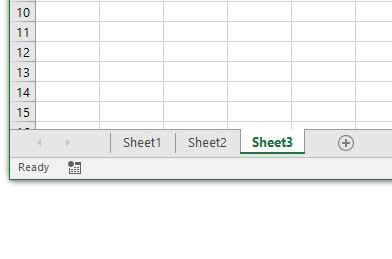
Step 2: Locate the worksheet tab that you want to rename at the bottom of the window.

Step 3: Right-click on the tab that you want to rename, then select the Rename option from the menu.

Step 4: Type the desired name for the tab, then press Enter on your keyboard.

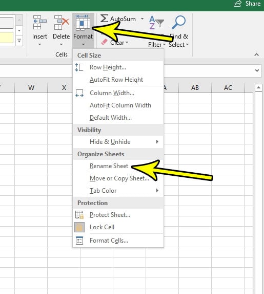
Note that you can also elect to rename an Excel tab by selecting the Home tab, clicking the Format button in the Cells section of the ribbon, then choosing the Rename Sheet option from that menu.

Our tutorial continues below with additional information on renaming sheet tabs in Excel.
How to Use the Excel Cell Function to Get a Sheet Name in an Excel Workbook
A useful function that you can employ in Microsoft Excel involves the use of the “CELL” function or formula. This is a helpful way to display a cell value in one of the cells of your current worksheet which contains just the sheet name of the current worksheet.
Using a function to display this information is useful because if the worksheet names ever change, then the related functions that contain all the sheet names will update to reflect that change.
If you click inside a cell where you want to display a sheet tab name you can type the formula:
=CELL(“FILENAME”,A1)
The worksheet name will then be displayed at the end of the filepath. Note that you need to save the file first before it will display this information.
Why Don’t I See Any Sheet Tabs in Excel?
While the worksheet tabs are visible at the bottom of the window in Excel by default, it is possible to hide them. This is often done so that other people viewing the file can’t see those tabs and edit them. Someone may also choose to hide worksheet tabs because they want the extra visible spreadsheet area on their screen.
If all of your worksheet tabs are hidden, including the one for the worksheet that is currently the active sheet, then you are going to need to change a setting on the Excel Options menu.
- Click the File tab.
- Choose Options at the bottom-left.
- Select the Advanced tab.
- Scroll down to the Display options for this workbook section.
- Check the box to the left of Show sheet tabs.
- Click OK.
If you can see at least one sheet tab, however, then you are going to need to unhide your worksheet tabs in a different manner. That is discussed in the next section.
How to Hide or Unhide a Sheet Tab in Excel
As we mentioned in the previous section, hiding a worksheet tab can be a quick way to make it more difficult for someone to edit or change information that appears on a worksheet. For example, if you have formulas in your worksheets that are referencing important data or constant data that shouldn’t be changed, then putting them on a separate worksheet and hiding it can be effective in stopping other people from finding or editing it.
You can hide a worksheet tab by right-clicking on the tab at the bottom of the window, then choosing the Hide option.
If you have a hidden tab that you need to display, then you can right-click on any of the tabs at the bottom of the window and choose the Unhide option. You can then select that worksheet and click the OK button. If you have multiple worksheet tabs that you want to unhide at the same time then you can hold down on the Ctrl key and click each worksheet on the Unhide window before you click the OK button.
More Information on How to Change a Tab Name in Excel 2016
The steps in the article above showed you how to name a tab in Excel. This can be useful not only for you as the editor of your Excel workbook, but for other people that need to look at your data or work on the file.
Additionally, the tab name or worksheet name in Excel can be added automatically to the head or footer of the page, if that is information that you would like to place in that location for when you print the worksheet in the future.
You can add the worksheet name to the header or footer by selecting the Page Layout tab at the top of the window, clicking the small Page Setup button at the bottom-right of the Page Setup group in the ribbon, then selecting the Header/footer tab. You can then click the Custom Header or Custom Footer button and add the tab name to one of the sections of that location by clicking the Insert Sheet Name button.
The reference tab name and the workbook name can also be useful when you are trying to reference other Excel sheet cells. When you are typing a formula in the current sheet and need to reference information in other sheets, then typing that formula can be much simpler if the rest of the worksheets in the current workbook have tab names that make sense.
One of the best things that you can do when you print a spreadsheet in Excel 2016 is to change some settings to make your data easier to read on paper. One such change involves repeating the top row on every page. This makes it easier for readers to identify columns and reduces the likelihood that they will identify a cell’s column incorrectly.
Additional Reading

Kermit Matthews is a freelance writer based in Philadelphia, Pennsylvania with more than a decade of experience writing technology guides. He has a Bachelor’s and Master’s degree in Computer Science and has spent much of his professional career in IT management.
He specializes in writing content about iPhones, Android devices, Microsoft Office, and many other popular applications and devices.