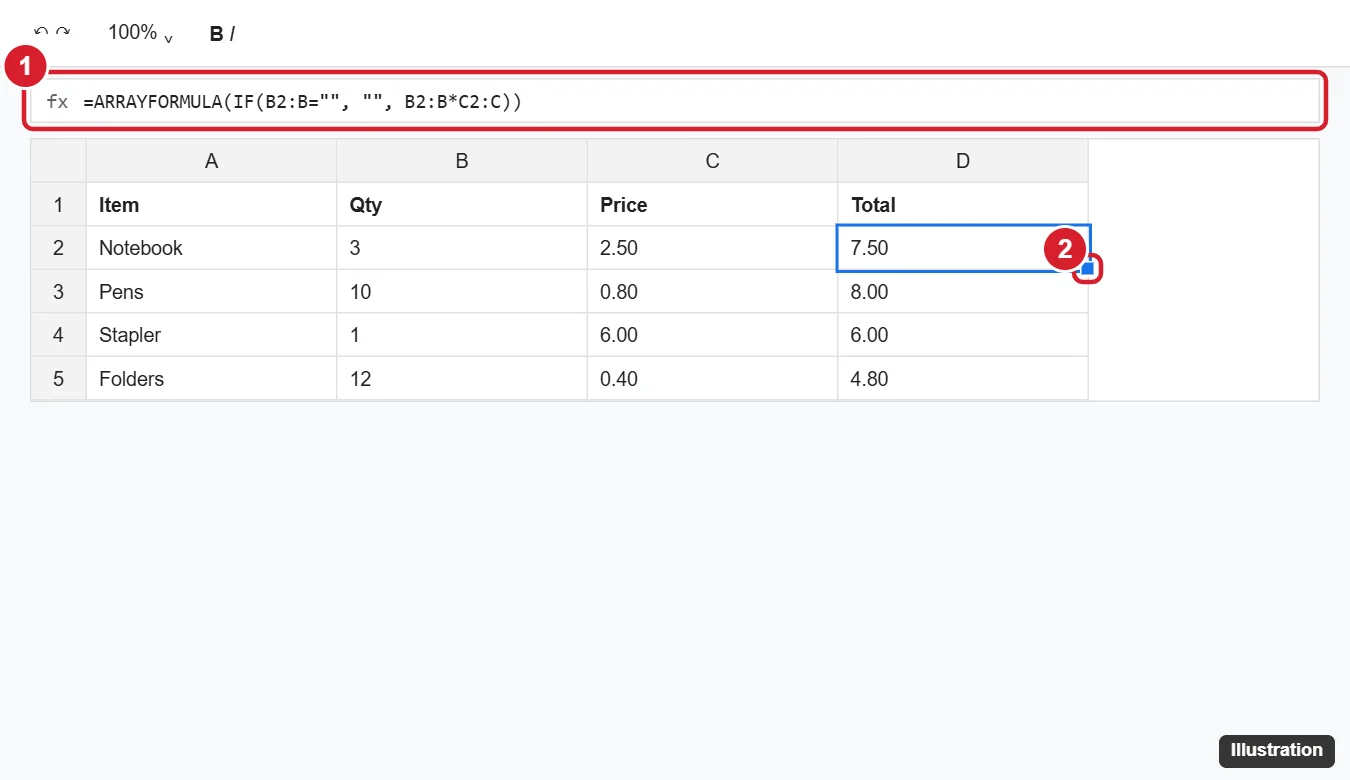
The fastest way to apply a formula to an entire column in Google Sheets is to type the formula in the first cell (for example, =B2*C2 in D2), select that cell, and double-click the fill handle (the small blue square in the cell’s bottom-right corner). Sheets copies the formula down to the last row of adjacent data. For a single formula that covers the whole column automatically, including new rows, use ARRAYFORMULA, such as =ARRAYFORMULA(IF(B2:B="", "", B2:B*C2:C)).
This guide covers every method, when to use each, how to lock references with dollar signs, and fixes for common errors like #REF! and formulas that don’t update.
Method 1: Double-click the fill handle
- Type the formula in the first data row, such as D2.
- Click the cell to select it.
- Double-click the small blue square in the bottom-right corner. The formula fills down as far as the data in the neighboring column goes.
Google Sheets may also show an Autofill suggestion after you enter the first formula; press Ctrl + Enter (or click the check mark) to accept it.
Method 2: ARRAYFORMULA (one formula for the whole column)
- Click the first result cell, such as D2, and make sure the cells below it are empty.
- Type a formula using whole-column ranges, for example
=ARRAYFORMULA(B2:B*C2:C). - Wrap it in IF to leave blank rows empty:
=ARRAYFORMULA(IF(B2:B="", "", B2:B*C2:C)). - Press Enter. Results spill down the column and update as you add rows.
Shortcut: type the formula and press Ctrl + Shift + Enter to wrap it in ARRAYFORMULA automatically.
Method 3: Select the range and press Ctrl + Enter
- Select the range where you want the formula, such as D2:D500 (click D2, then press Ctrl + Shift + Down arrow if the column has data, or type the range in the Name box).
- Type the formula for the first row.
- Press Ctrl + Enter to fill every selected cell with the adjusted formula.
Method 4: Copy and paste or Ctrl + D
- Copy the first formula cell (Ctrl + C), select the rest of the column, and paste (Ctrl + V).
- Or select the formula cell plus the empty cells below it and press Ctrl + D to fill down.
Lock references with dollar signs
When copying formulas, cell references shift. To keep one fixed, such as a tax rate in F1, write $F$1 (press F4 while editing a reference to cycle through options). Example: =B2*$F$1.
Which method should I use?
| Method | Best for |
|---|---|
| Fill handle | Quick, one-time fills next to existing data |
| ARRAYFORMULA | Columns that grow, such as form responses |
| Ctrl + Enter | A specific range, including non-adjacent data |
| Copy/paste or Ctrl + D | Small ranges or mixed data |
Troubleshooting
- #REF! with ARRAYFORMULA – “Array result was not expanded” means cells below have data. Clear them.
- Fill handle stops early – the neighboring column has a blank cell. Select the range manually instead.
- Formula shows as text – the cell is formatted as Plain text. Change Format > Number > Automatic and re-enter it.
- Slow sheet – very large ARRAYFORMULA ranges can slow things down; limit the range, such as B2:B1000.
Frequently asked questions
How do I apply a formula to an entire column including the header?
Put a formula in the header row that uses IF(ROW(…)=1, “Header”, …) with ARRAYFORMULA, or keep the header as text and start the formula in row 2.
Does this work on the Sheets mobile app?
Yes. Tap the cell, tap the blue handle, and drag down, or enter an ARRAYFORMULA.
Is it the same in Excel?
Mostly. Excel also supports double-clicking the fill handle, and newer versions spill array formulas automatically.

Kermit Matthews is a freelance writer based in Philadelphia, Pennsylvania with more than a decade of experience writing technology guides. He has a Bachelor’s and Master’s degree in Computer Science and has spent much of his professional career in IT management.
He specializes in writing content about iPhones, Android devices, Microsoft Office, and many other popular applications and devices.