How to Search for a Word in Google Sheets

In a large Google Sheets spreadsheet, scrolling to find a name, order number, or keyword is slow. The built-in search finds every match instantly, and Find and replace can search every tab, match exact case, or even look inside formulas. This guide covers quick search, advanced options, formulas that find words for you, and searching on your phone.

Quick Answer

Press Ctrl + F (Command + F on Mac) and type the word. Matching cells are highlighted, and you can press Enter to jump between them. For more options, like searching all sheets, press Ctrl + H to open Find and replace.

Method 1: Quick Search (Current Sheet)

1. Click anywhere in the spreadsheet.
2. Press Ctrl + F (Command + F). A search box appears at the top right.
3. Type the word. Matches are highlighted and a count appears (for example, 1 of 3).
4. Press Enter or use the arrows to move between matches. Press Esc to close.

Quick search looks only in the current sheet tab and ignores upper and lower case.

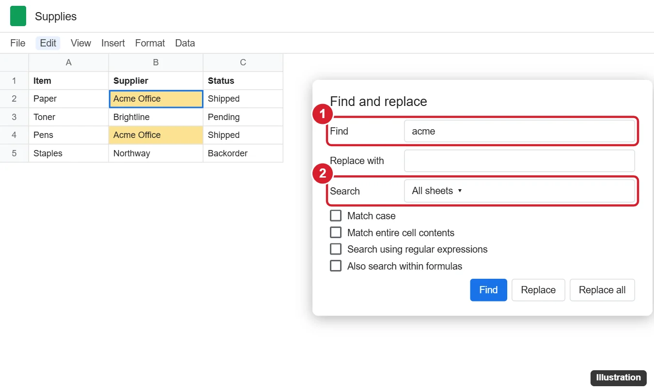
Method 2: Find and Replace (More Options)

1. Press Ctrl + H (Command + Shift + H on Mac), or go to Edit > Find and replace, or click the three dots in the quick search box.
2. Type the word in Find.
3. Under Search, choose All sheets, This sheet, or Specific range.
4. Optional settings:
   • Match case: finds “Acme” but not “acme.”
   • Match entire cell contents: finds cells that contain only that word.
   • Search using regular expressions: advanced patterns, like ^Acme for cells starting with “Acme.”
   • Also search within formulas: finds text inside formulas, not just their results.
5. Click Find repeatedly to step through matches. Enter text in Replace with and click Replace or Replace all to change them.

Method 3: Formulas That Find Words

• Count matches: =COUNTIF(A:C, “*acme*”) counts cells containing “acme” anywhere.
• List matching rows: =FILTER(A2:C, ISNUMBER(SEARCH(“acme”, B2:B))) shows every row where column B contains “acme.”
• Find a position: =MATCH(“Toner”, A:A, 0) returns the row number of an exact match.
• Look up related data: =XLOOKUP(“Toner”, A:A, C:C) returns the status for “Toner.”

Method 4: Highlight Every Match

To keep matches highlighted, select the range, go to Format > Conditional formatting, choose Text contains, type the word, pick a color, and click Done.

Method 5: Filter by a Word

Select your data and click Data > Create a filter. Click the filter icon in a column header, choose Filter by condition > Text contains, and type the word to show only matching rows.

Search on Your Phone

1. Open the spreadsheet in the Google Sheets app.
2. Tap the three dots and choose Find and replace.
3. Type the word and tap Search; use the arrows to move between results.

Making a quiz from existing questions? See how to import questions into Google Forms.

To mark what you find, color the cells with Fill color.

You can also remove checkboxes in bulk.

To total the matches, see how to count a word in Google Sheets.

Tracking tasks? See putting several checked choices in one cell.

Troubleshooting

• Word not found: Check for extra spaces or different spelling, turn off Match case and Match entire cell contents, and search All sheets.
• Found in the wrong place: The word may be in a formula result. Turn on Also search within formulas to search formula text.
• Hidden rows or columns: Matches in hidden rows may be skipped; unhide them first.

Summary

1. Press Ctrl + F to search the current sheet.
2. Press Ctrl + H to search all sheets with advanced options.
3. Use COUNTIF, FILTER, or conditional formatting to count, list, or highlight matches.