Alternating colors, sometimes called banding, shade every other row in Google Sheets. They are easy to add and just as easy to remove, but they live in their own panel rather than in the regular fill color menu, which is why clearing the fill color often does not work.
Quick Answer
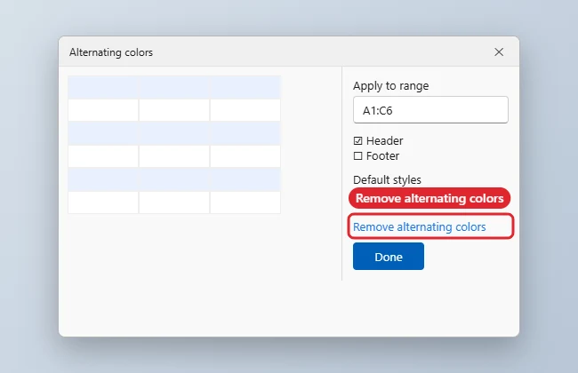
Select a cell in the banded range, choose Format, Alternating colors, and click Remove alternating colors at the bottom of the side panel.
How to Remove Alternating Colors in Google Sheets
- Click any cell inside the range with alternating colors.
- Open the Format menu and choose Alternating colors.
- In the side panel, check that Apply to range shows the right cells.
- Click Remove alternating colors at the bottom of the panel.
- If shading remains, look for conditional formatting in Format, Conditional formatting, and delete that rule.
Why Rows Might Still Be Colored
| Cause | Fix |
|---|---|
| Alternating colors | Format, Alternating colors, Remove |
| Conditional formatting | Format, Conditional formatting, delete the rule |
| Manual fill color | Fill color, Reset |
| Table formatting | Convert the table back to a normal range |
Special Cases
Several banded ranges on one sheet
Each block of alternating colors is a separate range. Click inside each one and remove it in turn; removing one does not affect the others.
Data formatted as a table
If your data has a table name above it and drop-down chips in the header row, it is a Google Sheets table, which has its own colour settings. Use the table menu next to the table name to change its colours or convert it back to a normal range, then remove any remaining banding.
Files imported from Excel
Excel table styles often arrive in Google Sheets as ordinary fill colours rather than alternating colors. Select the cells and press Ctrl + \ (Format, Clear formatting) to remove them. This also clears fonts, borders and number formats, so reapply any you want to keep.
Want Different Stripes Instead?
To change rather than remove the stripes, open Format, Alternating colors and pick a new default style, or set custom colours for the header, colour 1 and colour 2. For more control, such as shading every third row, delete the alternating colors and use Format, Conditional formatting with a custom formula like =MOD(ROW(),3)=0. See also how to apply alternating colors to rows in Google Sheets.
Troubleshooting
- The Remove button is missing: the selected cell is outside the banded range. Click a cell inside it.
- Only part of the range was cleared: the sheet may have several banded ranges. Repeat for each.
- To add banding back later, see how to highlight every other row in Google Sheets.
- To strip all formatting, read how to clear formatting in Google Sheets.
Related: remove conditional formatting in Google Sheets.
Frequently Asked Questions
Does removing alternating colors delete my data?
No. Only the shading is removed.
Can I change the colors instead?
Yes. In the same panel, pick a default style or set custom colors.
Does Clear formatting remove banding?
Not always. Alternating colors are separate, so use the Remove option.
Summary
- Click inside the banded range.
- Open Format, Alternating colors.
- Click Remove alternating colors.
- Check for conditional formatting.

Kermit Matthews is a freelance writer based in Philadelphia, Pennsylvania with more than a decade of experience writing technology guides. He has a Bachelor’s and Master’s degree in Computer Science and has spent much of his professional career in IT management.
He specializes in writing content about iPhones, Android devices, Microsoft Office, and many other popular applications and devices.