Finding the average (mean) of a set of numbers in Google Sheets takes one formula: AVERAGE. Sheets also shows a quick average when you select cells, and it has variations for averaging only the cells that meet a condition, skipping zeros, or including text values. This guide covers all of them with examples you can copy.
Quick Answer
Click an empty cell, type =AVERAGE(B2:B6) (replace the range with your cells), and press Enter. For a quick look without a formula, select the cells and check the Avg value in the bottom-right corner.
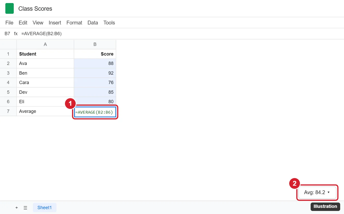
Method 1: The AVERAGE Function
- Click the cell where you want the result.
- Type
=AVERAGE(. - Drag over the cells to average, or type the range, such as
B2:B6. - Type
)and press Enter.
You can average separate ranges or individual cells too: =AVERAGE(B2:B6, D2:D6) or =AVERAGE(B2, B4, B6). AVERAGE ignores empty cells and text but includes zeros.
Method 2: Use the Functions Menu
- Select the cells you want to average (or the empty cell below them).
- Click the Functions button (Σ) on the toolbar.
- Choose AVERAGE. Sheets inserts the formula; adjust the range and press Enter.
Method 3: Quick Average Without a Formula
Select a range of numbers. The summary box in the bottom-right corner shows Sum by default; click it and choose Avg to see the average. This doesn’t add anything to the sheet.
Average with Conditions: AVERAGEIF and AVERAGEIFS
- One condition:
=AVERAGEIF(A2:A20, "East", C2:C20)averages sales in column C where the region in column A is “East.” - Numbers above a value:
=AVERAGEIF(C2:C20, ">50") - Multiple conditions:
=AVERAGEIFS(C2:C20, A2:A20, "East", B2:B20, ">=2026-01-01")averages East sales from 2026 onward.
Average Without Zeros
Use =AVERAGEIF(B2:B20, "<>0") to skip cells containing 0. This is useful when zeros mean “no data” rather than an actual score.
Other Averaging Functions
| Function | What it does |
|---|---|
AVERAGEA |
Counts text as 0 and TRUE as 1, FALSE as 0 |
AVERAGE.WEIGHTED |
Weighted average: =AVERAGE.WEIGHTED(B2:B6, C2:C6) with weights in C |
MEDIAN |
Middle value, less affected by outliers |
MODE |
Most frequent value |
TRIMMEAN |
Average after excluding a percentage of highest and lowest values |
Round the Result
Wrap the formula in ROUND to control decimals: =ROUND(AVERAGE(B2:B6), 1). Or keep the full value and use Format > Number or the decrease-decimal button to change how many decimals display.
Troubleshooting
- #DIV/0! error: the range has no numbers. Check the range or use
=IFERROR(AVERAGE(B2:B6), ""). - Numbers ignored: they may be stored as text (left-aligned). Select them and choose Format > Number > Number, or use Data > Data cleanup tools.
- Average seems too low: zeros are included. Use AVERAGEIF with “<>0” if that’s not what you want.
- Result changes when adding rows: use an open-ended range like
B2:Bto include new rows automatically (make sure the formula isn’t inside that range).
Related: Calculate correlation in Google Sheets.
Frequently Asked Questions
Does AVERAGE include blank cells?
No. Blank cells are skipped, but cells containing 0 are included.
How do I average an entire column?
Use =AVERAGE(B:B) in a cell outside column B, or =AVERAGE(B2:B) to skip a header.
Can I average across sheets?
Yes: =AVERAGE(Sheet1!B2:B10, Sheet2!B2:B10).
Summary
- Type
=AVERAGE(range)and press Enter. - Select cells and read Avg in the bottom-right for a quick check.
- Use
AVERAGEIForAVERAGEIFSfor conditions. - Use
"<>0"to skip zeros and ROUND to tidy decimals.

Kermit Matthews is a freelance writer based in Philadelphia, Pennsylvania with more than a decade of experience writing technology guides. He has a Bachelor’s and Master’s degree in Computer Science and has spent much of his professional career in IT management.
He specializes in writing content about iPhones, Android devices, Microsoft Office, and many other popular applications and devices.