The steps in this guide are going to show you the setting in Google Sheets that will let you add or remove the gray bar that runs horizontally or vertically between rows or columns in your spreadsheet. We cover the steps briefly at the top of the article, then continue further with additional information and pictures for the steps.
- Open your spreadsheet in Google Sheets.
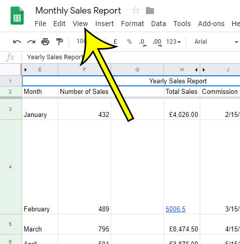
- Click the View tab at the top of the window.
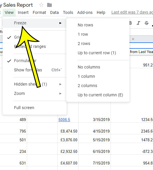
- Select the Freeze option, then choose No rows or No columns to remove the gray bar, or select one of the other options to add it.
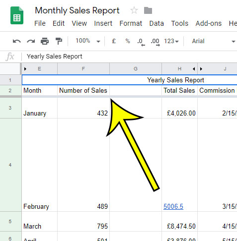
Are you working on a spreadsheet in Google Sheets and you see a thick gray bar either under one of your rows or to the right of one of your columns? This bar is an indication that some rows or columns in your spreadsheet are frozen. You can see the bar in the picture below.

Freezing rows in spreadsheet applications like Google Sheets or Microsoft Excel allows you to keep a row or column visible on the screen even when you scroll down or to the right. This is beneficial if that row or column contains important identifying information for your cells.
Our tutorial below will show you where to find the Menu that lets you control whether or not your rows or columns are frozen. This menu will let you remove the gray bar if you don’t want or need it, or it will let you customize which rows or columns are frozen on the sheet.
Our guide on how to make all columns the same width in Google Sheets can show you a simple way to evenly distribute your spreadsheet columns.
How to Add or Remove the Gray “Freeze” Bar in Google Sheets
The steps in this guide were performed in the desktop version of the Google Chrome Web browser, but will also work in other desktop browsers like Mozilla Firefox or Microsoft Edge.
Step 1: Sign into your Google Drive at https://drive.google.com and open the spreadsheet that you wish to edit.
Step 2: Select the View tab at the top of the window.

Step 3: Choose the Freeze option, then select No rows or No columns to remove the gray bar.

If you would like to freeze some of your rows or columns, simply select the option that matches the range that you wish to freeze.
Find out how to add a drop down menu in Google Sheets and make it a little easier to add the same set of information to a row or column.

Kermit Matthews is a freelance writer based in Philadelphia, Pennsylvania with more than a decade of experience writing technology guides. He has a Bachelor’s and Master’s degree in Computer Science and has spent much of his professional career in IT management.
He specializes in writing content about iPhones, Android devices, Microsoft Office, and many other popular applications and devices.