Hiding data in an Excel spreadsheet is a common practice when there is data that isn’t necessary to view, but that you either need for a formula, or aren’t sure that you actually want to delete.
Perhaps you have even hidden some rows or columns before, and like the ability to streamline the data that is visible when you are working in Excel.
But people also have a tendency to hide entire worksheets. I find that I often do this when I have a sheet that contains important information that I don’t want people to edit.
If you have a workbook that contains a hidden worksheet that you need to either be able to view or edit, then our guide below will show you how to unhide it.
How to Unhide a Sheet in Excel
The steps in this article were performed in Microsoft Excel 2013, but you can use the same steps to unhide a worksheet tab in Excel 2013. Note that you will be able to unhide any hidden worksheet in your workbook, regardless of which tab you right-click on.
Step 1: Open the workbook containing the worksheet tab that you want to unhide.
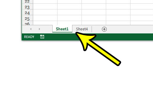
Step 2: Locate the worksheet tabs below the spreadsheet. If you don’t see any tabs in that location, then you might need to change an Excel setting. This article will show you where to find the setting that you need to adjust.

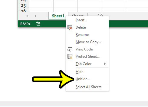
Step 2: Right-click one of the worksheet tabs, then select the Unhide option.

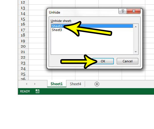
Step 3: Click the worksheet that you want to unhide, then click the OK button.

Now that you know how to unhide a worksheet in Excel 2013, you can easily find previously-hidden sheets so that you can edit data contained within them.
Are you having difficulty printing your spreadsheets? Read our guide to Excel printing for some useful settings in the program that can make it a lot easier to print spreadsheets, especially large ones that have a tendency to spill over onto additional unwanted pages.

Kermit Matthews is a freelance writer based in Philadelphia, Pennsylvania with more than a decade of experience writing technology guides. He has a Bachelor’s and Master’s degree in Computer Science and has spent much of his professional career in IT management.
He specializes in writing content about iPhones, Android devices, Microsoft Office, and many other popular applications and devices.