If you have ever opened the Format Cells window in Microsoft Excel and explored the sections in there then you might have discovered a Font tab that includes a number of different ways that you can customize text. Included among these is an option that you can use if you need to know how to remove strikethrough in Excel, or if you want to add a line through your text instead.
Using the strikethrough effect in documents is helpful for letting a reader know that the text has been removed, while still leaving it there as a reference in case it is needed later. This formatting option is available in Microsoft Excel and is used occasionally for a number of reasons.
If you are editing a document in Excel 2013 and encounter cells that contain text with the strikethrough effect, then you might be trying to figure out how to get rid of it. Our guide below will show you where to find the strikethrough setting in Excel 2013 so that you can remove that formatting.
How to Get Rid of Strikethrough in Excel
- Open your spreadsheet.
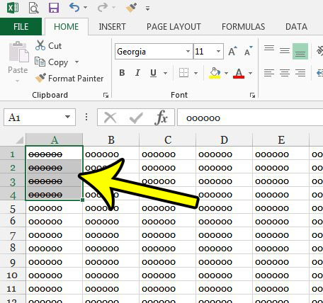
- Select the cells to modify.
- Choose the Home tab.
- Click the Font Settings button.
- Uncheck Strikethrough, then click OK.
Our guide continues below with additional information on removing strikethrough in Excel 2013, including pictures of these steps.
How to Remove a Line Through Text in Excel 2013 (Guide with Pictures)
The steps in this article were performed in Microsoft Excel 2013. This guide assumes that you currently have text in your spreadsheet that has a line going through it. Our steps below are going to show you how to select the cells containing the strikethrough effect, then remove that effect.
Step 1: Open your spreadsheet in Excel 2013.
Step 2: Select the cells containing the strikethrough text that you wish to remove.
If you would like to remove all of the strikethrough from your spreadsheet, click the cell above the row 1 heading and to the left of the column A heading.

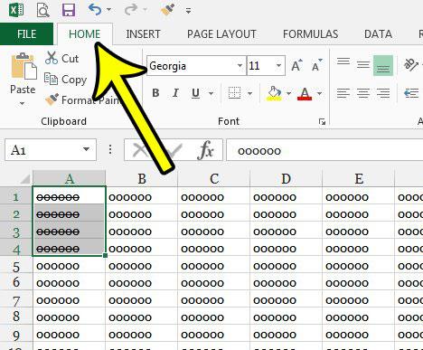
Step 3: Click the Home tab at the top of the window.

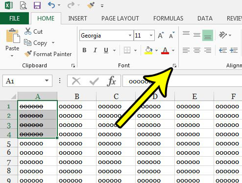
Step 4: Click the Font Settings button at the bottom-right corner of the Font section of the ribbon.

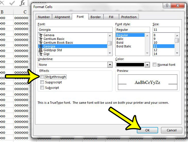
Step 4: Click the box to the left of Strikethrough to remove the check.
I have removed strikethrough from my selected text in the image below. Click the OK button at the bottom of the window to apply the change.

Our tutorial continues below with additional information on removing the line through text in Microsoft Excel.
More Information on How to Remove Strikethrough in Excel 2013
The steps above show you how to select text in your Excel spreadsheet and remove any strikethrough formatting that has been applied to it. Another way to add strikethrough is with a keyboard shortcut. After you have selected cells where you want to add a line through text or remove a line through text, simply press Ctrl + 5 on your keyboard. Shortcuts like this are very useful in Microsoft Office applications, particularly when you are performing an action that you use a lot.
You can use a similar method if you want to draw a line through your text. Simply select the text that you would like to strikethrough, then go to Home > Font Settings and check the Strikethrough box. Once you are done you can click OK to close the Format Cells dialog box, then Excel will add strikethrough to the selected text. Note that you can use this same method if you want to apply strikethrough to multiple cells. You just first need to select all the cells where you want to add the strikethrough option, then click the Font Settings button in the Font group of the ribbon and check the Strikethrough button.
This same method can be applied to add or remove superscript or subscript formatting as well.
In other applications, such as Google Sheets, you need to select the entire cell or cells to which you want to add the line through text, then you can simply select Strikethrough in the toolbar above the spreadsheet.
If you want to select an entire row or an entire column then you can click the row number to the left of the spreadsheet or the column letter at the top of the spreadsheet to select each cell in that range. If you want to select random, not adjacent cells then you need to hold the Ctrl key on your keyboard as you click each of those cells. If you need to select a range of adjacent cells then, rather than press Ctrl, select the first cell, then press the Shift key and click the last cell. All of the cells between those two cells should then be selected.
If you select cells that contain a combination of text with strikethrough and text without a line through it, then you may need to click the check box next to Strikethrough a couple of times until it is empty.
Are there other types of formatting applied to your cells that you would like to remove? Learn about a quick way to clear formatting in Excel 2013 so that you don’t need to go through and manually adjust every type of formatting that has been applied.

Kermit Matthews is a freelance writer based in Philadelphia, Pennsylvania with more than a decade of experience writing technology guides. He has a Bachelor’s and Master’s degree in Computer Science and has spent much of his professional career in IT management.
He specializes in writing content about iPhones, Android devices, Microsoft Office, and many other popular applications and devices.