Storing and analyzing data in Excel is something that almost every business will need to do. Whether you are tracking product sales, revenue, or website statistics, Excel provides a useful means for looking at, editing, and sorting that information.
Occasionally some values in your spreadsheet will be negative, and they are likely formatted with a preceding “-” to indicate that the number is read.
But if you are simply reading that data, it can be very easy to misidentify a negative number as a positive number. One helpful way to minimize the risks of this occurring is to make all of the negative numbers in a row or column red.
Our guide will show you how to apply red formatting to negative numbers in Excel 2013 to make those negative numbers stand out amidst the positive numbers that surround them.
How to Automatically Format All Negative Numbers with Red Text in Excel 2013
The steps below are going to show you how to format your selected cells so that any negative numbers displayed within those cells will display with red text.
Step 1: Open your spreadsheet in Excel 2013.
Step 2: Select the column letter, row number, or group of cells containing the numbers that you would like to format with red text.
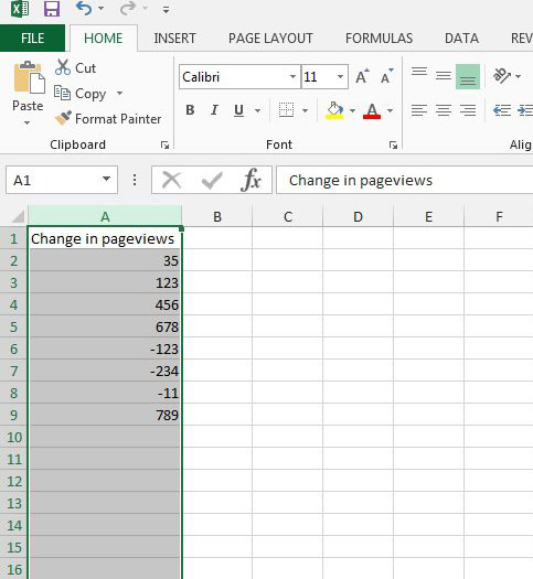
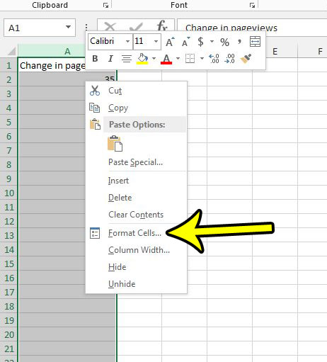
Step 3: Right-click any of the selected cells, then click the Format Cells option.
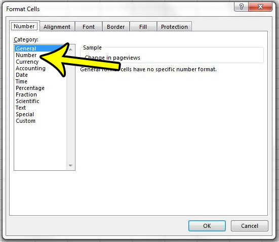
Step 4: Click the Number option under Category at the left side of the window.
Step 5: Select one of the red text options under Negative numbers, then click the OK button.
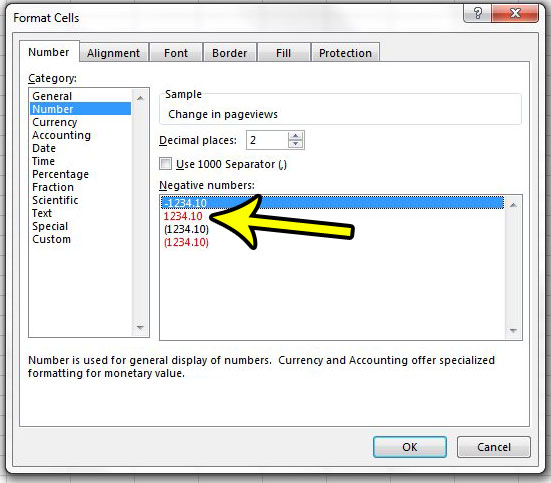
Any negative numbers in your selected cells should now be red. If there are decimal places after your numbers and you don’t want them there, simply return to the menu in Step 5 and change the value in the Decimal places field to 0.
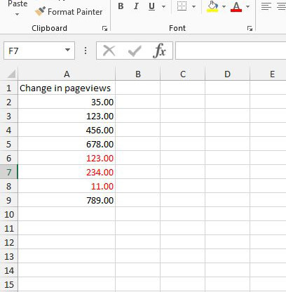
Now that you know how to make all negative numbers red in Excel 20103, you will find that it is easier to identify those values in the cells in your spreadsheets.
Summary – Using Red for Negative Excel Numbers
- Open Excel.
- Select the cells ot change.
- Right-click on a selected cell and choose Format Cells.
- Select the Number category.
- Choose a red number option, then click OK.
Are you trying to print your spreadsheet, but it’s difficult to read on a printed page? Read our guide to printing from Excel and learn about some really useful settings that can make printing your spreadsheets a lot easier for you and the people that read those spreadsheets.

Kermit Matthews is a freelance writer based in Philadelphia, Pennsylvania with more than a decade of experience writing technology guides. He has a Bachelor’s and Master’s degree in Computer Science and has spent much of his professional career in IT management.
He specializes in writing content about iPhones, Android devices, Microsoft Office, and many other popular applications and devices.