While strikethrough is not something that a lot of people use, it can become really useful once you become comfortable with that type of formatting.
You may already know how to draw a line through text in Google Docs or other word processing applications, but it’s also possible to draw lines through text in Excel spreadsheets.
Our tutorial below will show you where to find this option and use it on the data in your cells.
How to Strikethrough Excel 2013
- Open the file.
- Select the cell to strikethrough.
- Click Home.
- Click Font Settings.
- Check the Strikethrough box, then click OK.
Our article continues below with additional information on how to draw line through text in Excel 2013, including pictures of these steps.
The ability to strikethrough in Excel can come in handy when you need to format cells text in Excel in a way that keeps that text in the spreadsheet, but indicates that it should be ignored.
Microsoft Excel has a large number of different ways to adjust the appearance of data in your cells, and the strikethrough formatting is one of those options, though it can be tough to find.
The strikethrough effect is a helpful thing to use when you are creating documents. It provides you with a way to visually delete or mark information as something that is not important, but it allows you to keep it around so that readers can still see it, or in case you decide later that you need it.
The strikethrough effect is particularly helpful when you are working with data in a spreadsheet, so you might be looking for a way to use that formatting option in Excel 2013.
Our guide below will show you how to find the strikethrough option both through the ribbon, as well as a shortcut that you can use to quickly draw or remove a line through cell data.
How to Draw a Line Through Numbers or Text in Excel 2013 (Guide with Pictures)
The steps in this guide are going to show you how to draw a line, also called “strikethough”, through information contained within a cell in your Excel spreadsheet.
While this guide will be focused specifically on doing this to one cell, you can choose any number of cells that you would like.
Step 1: Open your spreadsheet in Excel 2013.
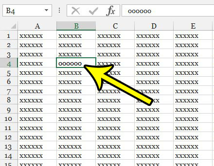
Step 2: Select the cell to which you want to apply the strikethrough effect.

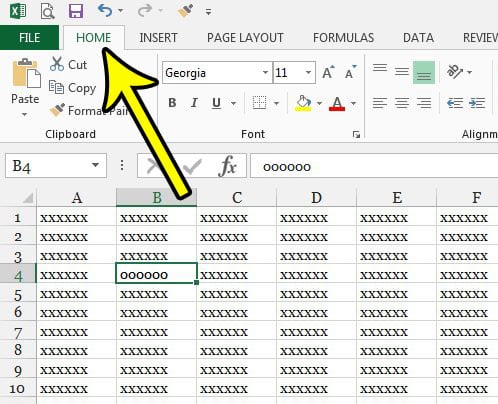
Step 3: Click the Home tab at the top of the window.

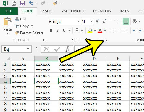
Step 4: Click the small Font Settings button at the bottom-right corner of the Font section in the ribbon.

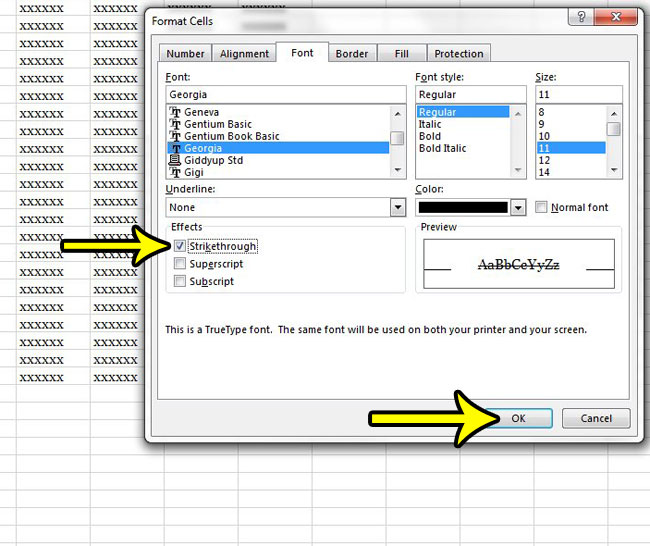
Step 5: Check the box to the left of Strikethrough, then click the OK button.

Now that you have completed our draw line through text in Excel steps, you will be able to use or remove this formatting in the cells in your spreadsheets.
You can use these same steps to remove strikethrough in a cell. You will just want to click the box to remove the check mark.
Additionally, the strikethrough effect can be applied or removed by simultaneously pressing the Ctrl + 5 keys on your keyboard. That is the keyboard shortcut for Strikethrough in Excel 2013.
Is there a lot of formatting applied to your spreadsheet that you don’t want? Rather than changing each individual formatting option, learn how to clear cell formatting in Excel 2013 and save yourself some time and frustration.
Additional Information on How to Format Cells with Strikethrough in Excel
Strikethrough in Excel is particularly useful as a visual aid. You can still use strikethrough text or numbers in formulas, so feel free to draw a line through any text in Excel that you might be considering removing or that other viewers might want to ignore.
As mentioned above, the keyboard shortcut to strikethrough text is Ctrl + 5. Since getting to the Font dialog box to locate the strikethrough text option is a little cumbersome, then this keyboard shortcut is especially useful if you are going to format cells in this way on a regular basis.
While we focus specifically on how to apply the strikethrough effect to a single cell in our guide above, the same options can be used for multiple cells at once.
Simply select the cells that you want to strikethrough in Excel 2013, then use the menu option or the keyboard shortcut option described above. Note that you can format cells in other ways, too, when multiple cells are selected. The fastest way to select all of the cells in your spreadsheet is to press Ctrl + A on your keyboard or to click the gray button above the row 1 heading and to the left of the column A heading.
Other Microsoft Office programs like Microsoft Word, Microsoft Outlook, and Microsoft Powerpoint will also let you use the strikethrough option to format text.
If you have never used one of the small buttons on the ribbon to open a dialog box, then you may be having trouble finding it. The picture in Step 4 above shows the button that you need to click. It’s at the bottom right corner of the Font tab, and it says Font Settings when you hover over it.

Kermit Matthews is a freelance writer based in Philadelphia, Pennsylvania with more than a decade of experience writing technology guides. He has a Bachelor’s and Master’s degree in Computer Science and has spent much of his professional career in IT management.
He specializes in writing content about iPhones, Android devices, Microsoft Office, and many other popular applications and devices.